這頁是 ISF / phase noise / jitter 的動手例題庫。理論頁教你公式怎麼來,這裡教你
把數字代進去、算到底、檢查單位、用一行 Python 驗證。所有公式都從
[AUTHORING_SPEC 權威公式表] 逐字沿用,數值以
numerical_feeling 與規範第 8 節 canonical
為主(qmax=1 pC、Γrms=0.5、f0=5 GHz、L(1MHz)=−100 dBc/Hz)。
怎麼用這頁:先遮住「逐步解」,自己算一遍,再對答案。類比設計師的核心能力是
在白板上估數量級——看到「−100 dBc/Hz @ 1 MHz、5 GHz」要能 30 秒內喊出
「幾百 fs jitter」。每題最後的 Python 一行只用來「驗算」,不是用來「代替手算」。
分四級:
- (A) 基礎換算:rad ↔ fs、dBc ↔ linear、phase PSD ↔ L。練到變反射動作。
- (B) ISF → phase noise:Eq.(21)/(23)/(24) 代數,把 Γrms,c0,qmax 代成 dBc/Hz。
- (C) jitter 積分:由 L(f) 積分得 σt;period jitter 的高通核。
- (D) 設計反推:要 −120 dBc/Hz 需多大 qmax/Γrms;ring 級數 N 怎麼選。
每題格式固定:題目 → 逐步解(帶單位)→ 結果 → dimension check → 一行 Python 驗證。
Python 都引用 simulations/common/ 的真實函式(見規範第 5 節 API),可直接跑。
A 級:基礎換算
這一級只有兩條核心關係,務必背到底:
Δt=2πf0Δϕ,Llinear=10LdBc/Hz/10,Sϕ=2Llinear.
例 A1:phase → time(1 mrad 在 5 GHz 是幾 fs?)
題目:f0=5 GHz、Δϕ=1 mrad,求 timing error Δt。
逐步解
第 1 步,寫出 phase→time 換算(規範公式 17,Δt=Δϕ/(2πf0))。2πf0 的單位是
rad/s(角頻率),Δϕ 是 rad,相除得秒:
Δt=2πf0Δϕ=2π×5×109 rad/s1×10−3 rad.
第 2 步,算分母:2π×5×109=3.1416×10¹⁰ rad/s。
Δt=3.1416×101010−3 s=3.183×10⁻¹⁴ s=31.8 fs.
結果:Δt≈31.8 fs。
Dimension check:[rad]/[rad/s]=[s] ✓。手感記憶點:5 GHz 下「1 mrad ≈ 32 fs」;
反過來「1 rad ≈ 31.8 ps」(剛好同樣的 31.83 數字,差 103 倍級)。週期 T=200 ps,所以
1 mrad 約是週期的 1.6×10⁻⁴。
Python 驗證
from simulations.common.noise_utils import phase_to_time_error
print(phase_to_time_error(1e-3, 5e9) * 1e15, "fs")
例 A2:dBc/Hz → linear(−100 dBc/Hz 是多少?)
題目:L=−100 dBc/Hz,換成 linear(每 Hz 相對載波的功率比),再還原 phase PSD Sϕ。
逐步解
第 1 步,dBc/Hz 是 10log10(⋅) 的「分貝相對載波」單位,反運算除以 10 再取 10 的次方:
Llinear=10L/10=10−100/10=10−10 [1/Hz].
第 2 步,小角單音 PM 近似下 L(f)≈21Sϕ(f)(規範公式 16 與第 10.2 節
「L≈21Sϕ」推導),故反推 phase PSD:
Sϕ=2Llinear=2×10⁻¹⁰ rad2/Hz.
結果:Llinear=10−10/Hz、Sϕ=2×10−10 rad²/Hz。
Dimension check:dBc/Hz 是無因次功率比 per Hz;Llinear 也是 1/Hz;乘 2 後當 phase PSD
讀作 rad²/Hz(rad² 是相位方差的單位,方差密度對 f 積分後得 rad²)✓。口訣:每 −10 dB
= 線性少一個數量級;每 −20 dB = 電壓/相位幅度少一個數量級。
Python 驗證
import numpy as np
from simulations.common.noise_utils import phase_psd_to_l_dbc_per_hz
s_phi = 2 * 10**(-100/10)
print(s_phi, "rad^2/Hz")
print(phase_psd_to_l_dbc_per_hz(s_phi), "dBc/Hz")
例 A3:injected charge → phase step → time(1 fC 踢一下)
題目(canonical 例 A):qmax=1 pC、Δq=1 fC、Γ=0.5、f0=5 GHz。
求單一脈衝造成的 phase step Δϕ 與 timing error Δt。
逐步解
第 1 步,用 ISF 操作型定義(規範公式 5,Δϕ=Γ(ω0τ)Δq/qmax)。
Γ 無因次、Δq/qmax 無因次,所以 Δϕ 是純數(rad):
Δϕ=qmaxΓΔq=1×10⁻¹² C0.5×(1×10−15 C)=5×10⁻⁴ rad.
換成度:5×10⁻⁴×π180≈0.0286∘。
第 2 步,用 A1 的換算轉成時間(f0=5 GHz):
Δt=2π×5×1095×10−4 s≈1.59×10⁻¹⁴ s=15.9 fs.
結果:Δϕ=5×10⁻⁴ rad(0.0286∘)、Δt≈15.9 fs。
Dimension check:Δϕ:[C]/[C]= 無因次 ✓;Δt:[rad]/[rad/s]=[s] ✓。
手感:1 fC ≈ 6240 個電子;在最敏感相位也只踢出 ~16 fs。單顆很小,但 noise 持續踢、
會被相位積分器累積(見 convolution_derivation)。
Python 驗證
from simulations.common.isf_utils import impulse_to_phase_step
from simulations.common.noise_utils import phase_to_time_error
dphi = impulse_to_phase_step(delta_q=1e-15, gamma_value=0.5, qmax=1e-12)
print(dphi, "rad ->", phase_to_time_error(dphi, 5e9)*1e15, "fs")
例 A4:相位敏感度隨注入相位變(LTV 的味道)
題目:理想 LC 振盪器 ISF 為 Γ(θ)=−sinθ。同樣 Δq=1 fC、qmax=1 pC,
分別在 zero-crossing(θ=π/2,波形斜率最大)與 peak(θ=0,波形頂點)注入,
求各自的 Δϕ。
逐步解
第 1 步,先取兩處 ISF 值。注意這裡的相位約定:V∝cosθ 時波峰在 θ=0、
zero-crossing(下降沿)在 θ=π/2,理想 LC 的 Γ=−sinθ:
Γ(θ=π/2)=−sin2π=−1,Γ(θ=0)=−sin0=0.
第 2 步,各代入 Δϕ=ΓΔq/qmax(Δq/qmax=10−15/10−12=10−3):
ΔϕZC=(−1)(10−3)=−1×10⁻³ rad,Δϕpeak=(0)(10−3)=0 rad.
結果:在 zero-crossing 注入 → −1 mrad(最大相位效應);在 peak 注入 → 0 rad(純改振幅、不改相位)。
Dimension check:兩者皆 []⋅[C]/[C]= rad ✓。這就是 LTV(線性時變)的本質:
同一個 impulse,效果取決於「踢在波形的哪個相位」。peak 處 Γ=0 是因為那裡只有徑向(振幅)
擾動、沒有切向(相位)分量,而振幅會被 restoring 拉回。見
impulse_to_phase_shift。
Python 驗證
import numpy as np
from simulations.common.isf_utils import gamma_lc_ideal, impulse_to_phase_step
for name, th in [("ZC", np.pi/2), ("peak", 0.0)]:
g = gamma_lc_ideal(th)
print(name, impulse_to_phase_step(1e-15, g, 1e-12), "rad")
B 級:ISF → phase noise(代數)
這一級反覆用三條招牌公式(全部 [P1],逐字沿用規範第 3 節):
- 白噪 1/f² [P1] Eq.(21), p.185:
L=10log10(qmax2Γrms2⋅4Δω2in2/Δf)
- flicker 1/f³ [P1] Eq.(23), p.185:含 c02 與 ω1/f/Δω 因子。
- 1/f³ corner [P1] Eq.(24), p.185:Δω1/f3=ω1/fc02/(2Γrms2)。
提醒:Eq.(21) 的分母是 4Δω2(SSB 記帳慣例)。時域乾淨推導會得到 2Δω2,
差的 2 倍是文獻上著名的小爭議,不影響 Γrms2/qmax2 scaling 與 −20 dB/dec 斜率。
詳見 white_noise_to_phase_noise。本頁一律用 [P1] 原式的 4Δω2。
例 B1:白噪 → L(canonical 例 B,逐位算到底)
題目:f0=5 GHz、Δf=1 MHz offset、qmax=1 pC、Γrms=0.5、
白噪 in2/Δf=Si=10−24 A²/Hz。用 Eq.(21) 求 L(1MHz)。
逐步解
第 1 步,把 offset 頻率換成角頻率:Δω=2πΔf=2π×106=6.283×10⁶ rad/s,
Δω2=3.948×10¹³ (rad/s)2。
第 2 步,算 Eq.(21) 括號內的值(先把無因次與帶單位部分分開):
qmax2Γrms2=(10−12)20.25=0.25×1024=2.5×10²³ C−2.
4Δω2Si=4×3.948×101310−24=1.579×101410−24=6.333×10−39 A2/Hz⋅s2.
第 3 步,相乘(單位下面再 check):
2.5×1023×6.333×10−39=1.583×10⁻¹⁵.
第 4 步,取 10log10:
L=10log10(1.583×10⁻¹⁵)=−148.0 dBc/Hz.
結果:L(1MHz)=−148.0 dBc/Hz。
Dimension check:括號內必須無因次(log 的引數)。
[C−2]⋅[A2Hz−1s2];用 A=C/s ⇒ A2=C2/s2,
Hz−1=s,整理 C−2⋅(C2/s2)⋅s⋅s2=C−2⋅C2⋅s−2⋅s3=s。
還差一個 1/s——它來自 PSD 的「per Hz」本質:結果是「每 Hz 的相對功率」,故引數實為 1/Hz,取 log 後是 dBc/Hz ✓。
(這就是為何單位很容易看走眼;記住「最終是 dBc/Hz」即可。)
手感:這是「單一理想白噪源」的下限。真實電路有多個 noise 源、cyclostationary、flicker,
實測會比這高出數十 dB。
Python 驗證
import numpy as np
Grms, qmax, Si = 0.5, 1e-12, 1e-24
dw = 2*np.pi*1e6
L = 10*np.log10((Grms**2/qmax**2) * (Si/(4*dw**2)))
print(round(L, 2), "dBc/Hz")
例 B2:用 Parseval 從 cn 求 Γrms,再算 L
題目:理想 LC 的 ISF 純粹是 Γ(θ)=−sinθ,即只有一階諧波 c1=1、其餘 cn=0。
(a)用 Parseval(Eq.(20))求 Γrms;(b)若 qmax=1 pC、Si=10−24、Δf=1 MHz,求 L。
逐步解
第 1 步(a),Parseval([P1] Eq.(20)):∑ncn2=2Γrms2。這裡 ∑ncn2=c12=1,故
2Γrms2=1 ⇒ Γrms=21≈0.707.
(直接驗:Γrms2=2π1∫02πsin2θdθ=21,亦得 Γrms=1/2 ✓。)
第 2 步(b),代 Eq.(21),Γrms2=0.5:
L=10log10((10−12)20.5⋅4×3.948×101310−24)=10log10(3.166×10⁻¹⁵)=−145.0 dBc/Hz.
結果:Γrms=0.707;L(1MHz)=−145.0 dBc/Hz。
Dimension check:Γrms 無因次(cn 無因次)✓;L 同例 B1,dBc/Hz ✓。
注意 Γrms=0.707 比 canonical 的 0.5 大,故 L 比 B1 高約 3 dB(10log10(0.5/0.25)=3 dB),
合理。
Python 驗證
import numpy as np
from simulations.common.isf_utils import gamma_lc_ideal, gamma_rms
theta = np.linspace(0, 2*np.pi, 100000, endpoint=False)
Grms = gamma_rms(theta, gamma_lc_ideal(theta))
print("Grms =", round(Grms, 4))
L = 10*np.log10((Grms**2/(1e-12)**2)*(1e-24/(4*(2*np.pi*1e6)**2)))
print(round(L, 2), "dBc/Hz")
例 B3:對稱性與 1/f³(c0 的角色)
題目:兩顆振盪器,白噪與 qmax 相同,ω1/f=2π×1 MHz。A 波形完全對稱(c0=0),
B 略不對稱(c0=0.2,c1=1)。問:哪顆有 close-in 1/f³ 上轉?在 Δf=10 kHz 各自的 1/f³ 貢獻如何?
逐步解
第 1 步,看 Eq.(23):1/f³ 區的 phase noise 正比於 c02。
L1/f3=10log10(qmax2c02⋅8Δω2Si⋅Δωω1/f).
第 2 步,對 A:c0=0⇒ 括號 =0⇒L1/f3→−∞ dBc/Hz(沒有 flicker 上轉,
1/f³ 區被完全抑制)。實務上不會真的 −∞(其他機制接手),但相對 B 可低非常多。
第 3 步,對 B:c0=0.2,有限值。用 Eq.(24) 比較兩者的 1/f³ corner:
Δω1/f3=ω1/f⋅2Γrms2c02.
對 B,∑cn2=c02+c12=0.04+1=1.04⇒Γrms2=0.52,故
Δω1/f3,B=ω1/f⋅2×0.520.04=ω1/f×0.0385.
即 B 的 1/f³ corner 在 ≈0.0385ω1/f=2π×38.5 kHz。對 A,corner →0。
結果:A(對稱、c0=0)沒有 1/f³ 上轉;B(c0=0.2)有,corner 約 38.5 kHz。
設計守則:靠波形對稱性壓低 c0,就能把 1/f³ corner 推到遠低於 device 的 ω1/f。
Dimension check:Eq.(24) 中 c02/Γrms2 無因次,乘 ω1/f(rad/s)得 rad/s ✓。
Python 驗證
import numpy as np
w_1f = 2*np.pi*1e6
for name, c0, c1 in [("A", 0.0, 1.0), ("B", 0.2, 1.0)]:
Grms2 = 0.5*(c0**2 + c1**2)
corner = w_1f * c0**2/(2*Grms2)
print(name, "1/f^3 corner =", corner/(2*np.pi)*1e-3, "kHz")
例 B4:白噪 floor 與 offset 的 −20 dB/dec 斜率
題目:沿用 B1 的振盪器(L(1MHz)=−148 dBc/Hz,1/f² 區)。問 Δf=10 MHz 時的 L?
(即把 offset 拉遠 10 倍。)
逐步解
第 1 步,Eq.(21) 中 L∝1/Δω2,取 log 後是 −20log10Δω+const,
即每 offset ×10,L 掉 20 dB(−20 dB/decade)。
第 2 步,Δf 由 1 MHz → 10 MHz(×10):
L(10MHz)=L(1MHz)−20log10(10)=−148−20=−168 dBc/Hz.
結果:L(10MHz)=−168 dBc/Hz。
Dimension check:−20log10(Δf2/Δf1) 的引數無因次(頻率比)✓,結果是 dB 差,加到 dBc/Hz 仍是 dBc/Hz ✓。
手感:1/f² 區「每 decade 掉 20 dB」是 phase noise 圖最常用的目視斜率;對照 1/f³ 區是 −30 dB/dec。
Python 驗證
import numpy as np
Grms, qmax, Si = 0.5, 1e-12, 1e-24
def L(df): return 10*np.log10((Grms**2/qmax**2)*(Si/(4*(2*np.pi*df)**2)))
print(round(L(1e6),2), round(L(10e6),2), "dBc/Hz",
"slope =", round(L(10e6)-L(1e6),1), "dB/dec")
C 級:jitter 積分
核心:phase noise 是頻域密度,jitter 是時域的 rms,兩者用「積分 + 開根號 + ÷(2πf0)」連起來
(規範公式 18、19):
σϕ2=∫f1f2Sϕ(f)df,σt=2πf0σϕ.
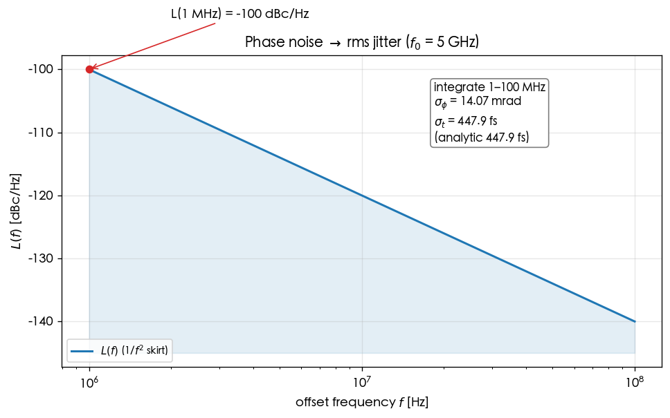
例 C1:L(f) → rms jitter(canonical 例 C,1/f² 積分)
題目:L(1MHz)=−100 dBc/Hz、1/f² 斜率、由 f1=1 MHz 積到 f2=100 MHz、
f0=5 GHz,求 σϕ 與 σt。
逐步解
第 1 步,把 datasheet 點換成 phase PSD(用 A2):Sϕ(fref)=2×10⁻¹⁰ rad²/Hz,fref=1 MHz。
第 2 步,寫 1/f² 形狀(以 fref 錨定):
Sϕ(f)=Sϕ(fref)(ffref)2=2×10⁻¹⁰(106)2f21.
第 3 步,積分(∫f−2df=−1/f):
σϕ2=2×10⁻¹⁰(106)2∫106108f2df=2×10²(1061−1081)=200×9.9×10−7=1.98×10⁻⁴ rad2.
故 σϕ=1.98×10−4=1.407×10⁻² rad =14.07 mrad。
第 4 步,換成 rms jitter(f0=5 GHz):
σt=2πf0σϕ=2π×5×1091.407×10−2≈4.48×10⁻¹³ s=447.9 fs.
結果:σϕ=14.07 mrad、σt=447.9 fs。
Dimension check:σϕ2:[rad2/Hz]⋅[Hz]=rad2 ✓;σt:[rad]/[rad/s]=[s] ✓。
手感:1/f² 積分被下限 f1 主導(1/f1≫1/f2)——「從哪裡開始積」對結果最關鍵。
若改成 −120 dBc/Hz @ 1 MHz(好 20 dB = 功率 1/100、幅度 1/10),jitter 縮到 ~45 fs。
Python 驗證
import numpy as np
from simulations.common.noise_utils import leeson_one_over_f2, integrate_rms_jitter
f = np.logspace(6, 8, 4000)
L = leeson_one_over_f2(f, L_ref_dbc=-100, f_ref=1e6)
sigma_t, sigma_phi = integrate_rms_jitter(f, L, f0=5e9, fmin=1e6, fmax=100e6)
print(round(sigma_phi*1e3,2), "mrad ;", round(sigma_t*1e15,1), "fs")
例 C2:積分下限主導——換下限會怎樣?
題目:同 C1 的譜(−100 dBc/Hz @ 1 MHz、1/f²、f0=5 GHz),但改成從 f1=100 kHz 積到 100 MHz。
估 σt,並和 C1 比較。
逐步解
第 1 步,1/f² 的 σϕ2∝(1/f1−1/f2)≈1/f1(下限主導)。下限由 106 變 105(小 10 倍),
1/f1 大 10 倍:
σϕ2≈2×10²(1051−1081)=200×(10−5−10−8)≈2.0×10⁻³ rad2.
第 2 步,σϕ=2.0×10−3=4.47×10⁻² rad =44.7 mrad(約 C1 的 10≈3.16 倍)。
第 3 步,σt=2π×5×1094.47×10−2≈1.42×10⁻¹² s =1.42 ps。
結果:σt≈1.42 ps(C1 是 448 fs)。下限降 10 倍 → jitter 約增 10≈3.16 倍。
Dimension check:同 C1 ✓。手感:這就是為什麼「rms jitter」一定要附上積分頻段才有意義;
量測儀器的下限(或 PLL 的迴路頻寬)決定你「看得到多少」累積 jitter。
Python 驗證
import numpy as np
from simulations.common.noise_utils import leeson_one_over_f2, integrate_rms_jitter
f = np.logspace(5, 8, 6000)
L = leeson_one_over_f2(f, L_ref_dbc=-100, f_ref=1e6)
sigma_t, sigma_phi = integrate_rms_jitter(f, L, f0=5e9, fmin=1e5, fmax=100e6)
print(round(sigma_phi*1e3,1), "mrad ;", round(sigma_t*1e12,2), "ps")
例 C3:period jitter 的高通核
題目:period jitter(單一週期長度的偏差 Tk−T)是相位的一階差分。用規範第 10.2 節的核
∣1−e−j2πfT∣2,對 C1 的譜(−100 dBc/Hz @ 1 MHz、1/f²、f0=5 GHz、T=200 ps)
估 period jitter σT。
逐步解
第 1 步,寫出 period jitter 公式(規範第 10.2 節 period/cycle-to-cycle 核):
σT2=(2πf0)21∫0∞Sϕ(f)∣1−e−j2πfT∣2df.
第 2 步,理解核的作用:∣1−e−j2πfT∣2=2(1−cos2πfT)=4sin2(πfT) 是高通——
低頻(fT≪1)被壓掉(∝f2),所以 period jitter 不被低頻 1/f² 的下限主導(和 C1/C2 的累積 jitter 相反)。
這就是為什麼 period jitter 通常比同譜的「accumulated jitter」小很多。
第 3 步,數值積分(手算不可行,直接交給電腦;常數已對齊規範核)。結果見下方 Python:σT≈27.6 fs。
結果:σT≈27.6 fs(對照 C1 的累積 σt=448 fs,小一個量級以上)。
Dimension check:核 ∣1−e−j2πfT∣2 無因次;∫Sϕ(核)df 得 rad²;
除 (2πf0)2 的 (rad/s)2… 注意這裡先得 rad² 再除 (2πf0)2 得 s²,開根號得 s ✓。
已解決(v5):period/cycle-to-cycle jitter 的確切前置常數已於 jitter_kernels 從第一性推導+Monte-Carlo 驗證(單邊 Sϕ 慣例下核為 4sin2,前置 1/ω02;本例 27.6 fs 即該頁閉式 28.28 fs 的截帶版本)
請對照標準文獻再確認;此處用規範第 10.2 節給的核,數值僅供量級手感。
Python 驗證
import numpy as np
T, f0, fref, Lref = 1/5e9, 5e9, 1e6, -100
f = np.logspace(3, 10, 2_000_000)
S_phi = 2 * 10**((Lref + 20*np.log10(fref/f))/10)
kernel = np.abs(1 - np.exp(-1j*2*np.pi*f*T))**2
trapz = getattr(np, "trapezoid", np.trapz)
sigma_T = np.sqrt(trapz(S_phi*kernel, f)) / (2*np.pi*f0)
print(round(sigma_T*1e15, 1), "fs")
例 C4:ring 累積 jitter σΔt=κΔt
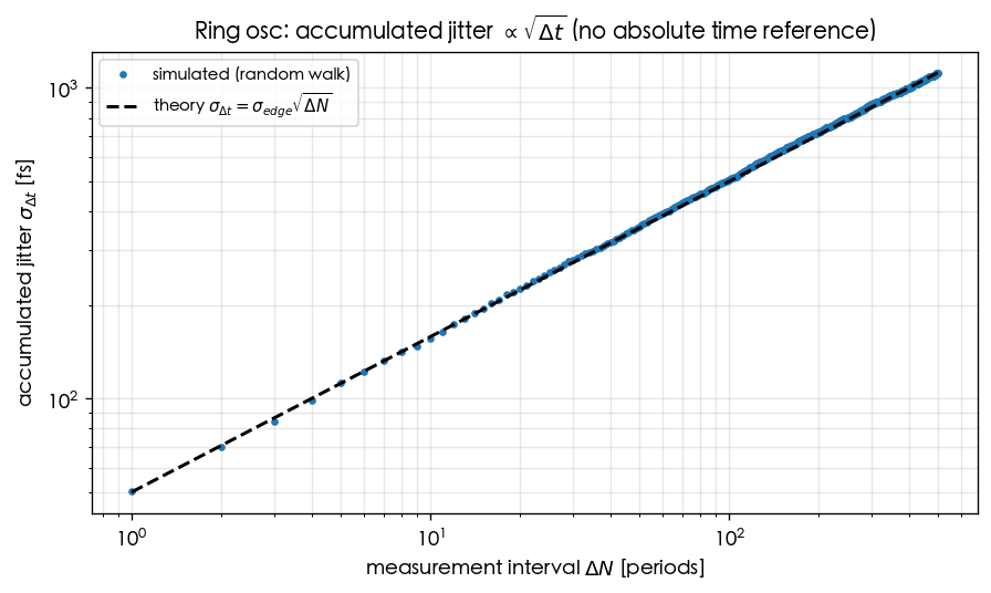
題目([P2] Eq.(8)):某 ring 的 jitter 比例常數 κ=1×10⁻⁸ s(toy 數值)。
求量測間隔 Δt=1 μs 與 Δt=1 ms 的累積 rms jitter。
逐步解
第 1 步,random-walk 律([P2] Eq.(8),無絕對時間參考的振盪器特徵):σΔt=κΔt。
第 2 步,Δt=10−6 s:
σΔt=10−810−6=10−8×10−3=10−11 s=10 ps.
第 3 步,Δt=10−3 s:
σΔt=10−810−3=10−8×3.162×10−2=3.16×10⁻¹⁰ s=316 ps.
結果:1 μs → 10 ps;1 ms → 316 ps。間隔 ×1000,jitter ×1000≈31.6。
Dimension check:κ 的單位 s,Δt 是 s,相乘得 s ✓
(這也是 κ 為何取那個怪單位的原因)。手感:ring(無高 Q tank)的相位是純隨機漫步,
等得越久誤差越大、且永不收斂——這正是 ring 比 LC 更「吵」的時域圖像。對照圖:
Python 驗證
import numpy as np
kappa = 1e-8
for dt in [1e-6, 1e-3]:
print(dt, "s ->", kappa*np.sqrt(dt)*1e12, "ps")
D 級:設計反推
把公式倒過來用:給規格,求需要多少 qmax、多小 Γrms、多少級 N。
例 D1:要 −120 dBc/Hz @ 1 MHz,qmax 要多大?
題目:規格 L(1MHz)=−120 dBc/Hz、f0=5 GHz。假設單一白噪源
Si=1×10⁻²¹ A²/Hz(比 canonical 大 1000 倍,較接近真實節點注入)、Γrms=0.5。
反推所需 qmax。
逐步解
第 1 步,從 Eq.(21) 解 qmax。先把規格換 linear:Llin=10−120/10=10−12。
10−12=qmax2Γrms2⋅4Δω2Si ⇒ qmax2=4Δω2LlinΓrms2Si.
第 2 步,代數值(Δω2=3.948×10¹³,Γrms2=0.25):
qmax2=4×3.948×1013×10−120.25×10−21=1.579×1020.25×10−21=1.583×10⁻²⁴ C2.
第 3 步,開根號:qmax=1.583×10−24=1.258×10⁻¹² C =1.26 pC。
結果:qmax≈1.26 pC(即把 canonical 的 1 pC 提升約 26%,配合此噪聲位準即可達標)。
Dimension check:qmax2:[]⋅[A2Hz−1]/([rad/s]2⋅[]);
用 A2Hz−1=C2s−2⋅s=C2s−1,除 s−2 得 C2s,
再吸收 PSD 的 per-Hz 後為 C2 ✓。設計手感:L∝1/qmax2,所以
qmax 加倍 → phase noise 降 6 dB。增大 qmax=CnodeVmax 的方法:加大擺幅 Vmax 或節點電容/電流。
Python 驗證
import numpy as np
Grms, Si, dw, Llin = 0.5, 1e-21, 2*np.pi*1e6, 10**(-120/10)
qmax = np.sqrt(Grms**2 * Si / (4*dw**2 * Llin))
print(round(qmax*1e12, 3), "pC")
例 D2:固定 qmax,要 −120 dBc/Hz 需多小 Γrms?
題目:同 D1 規格與噪聲(−120 dBc/Hz、Si=10−21、Δf=1 MHz、f0=5 GHz),但這次
qmax=1 pC 固定(不能再加大擺幅)。反推所需 Γrms。
逐步解
第 1 步,從 Eq.(21) 解 Γrms:
Γrms2=SiLlinqmax24Δω2=10−2110−12×(10−12)2×4×3.948×1013.
第 2 步,逐項算分子:10−12×10−24=10−36;×1.579×1014=1.579×10⁻²²。
除 10−21:Γrms2=0.1579。
第 3 步,Γrms=0.1579=0.397。
結果:Γrms≈0.40(須把 ISF rms 從 0.5 降到 0.40,約降 20%)。
Dimension check:Γrms2 無因次(同 B1 引數分析,所有帶單位項相消)✓。
設計手感:L∝Γrms2,Γrms 減半 → phase noise 降 6 dB。
降 Γrms 的手段:波形對稱(壓 c0)、把 noise 注入安排在 ISF 小的相位、ring 增加級數(見 D3)。
D1(調 qmax)與 D2(調 Γrms)是達同一規格的兩個獨立旋鈕。
Python 驗證
import numpy as np
qmax, Si, dw, Llin = 1e-12, 1e-21, 2*np.pi*1e6, 10**(-120/10)
Grms = np.sqrt(Llin * qmax**2 * 4*dw**2 / Si)
print(round(Grms, 3))
例 D3:ring 級數 N 的選擇(頻率 vs ISF)
題目:要做 f0=5 GHz single-ended ring。(a)若每級延遲 τD=20 ps,需幾級 N?
(b)若把級數從 N=5 增到 N=15(同時調 τD 維持 f0),用 Γrms∝N−3/2
估 phase noise 改變幾 dB(只看 Γrms 這個因子)?
逐步解
第 1 步(a),ring 頻率([P2] Eq.(15)):f0=2NτD1⇒N=2f0τD1。
N=2×5×109×20×10−121=0.21=5.
第 2 步(b),Γrms∝N−3/2([P2] Eq.(16), p.794,v7 已重核:根號只蓋常數,正文 4/N1.5@η=0.75 與 App.B Eq.(55) 三重驗證。v3 曾誤讀為 N−3/4;scaling 為主)。比值:
Γrms(5)Γrms(15)=(515)−3/2=3−1.5=0.1925.
第 3 步,phase noise ∝Γrms2,故改變量(dB):
ΔL=10log10(0.19252)=10log10(0.0370)=−14.3 dB.
結果:(a)N=5 級。(b)只看 Γrms 這一項,N 由 5→15 使 phase noise 低約 14.3 dB。
Dimension check:N=1/(2f0τD):1/([Hz][s])=1/([s−1][s])= 無因次 ✓
(N 應為整數,這裡剛好整)。ΔL:10log10 的引數是無因次比值 ✓。
重要警語:上面只孤立看了 Γrms。[P2] 的完整結論是——固定 f0 與總功率 P 時,
single-ended ring 的 phase noise / jitter 幾乎與 N 無關(見 [P2] Eq.(23), p.796 的 FOM,已核實)。
因為增加 N 雖降 Γrms,但同時 noise 源變多、每級擺幅/功率分配改變,互相抵消。
所以 D3(b) 的「14.3 dB」是只變一個因子的教學示意,不是真實設計可白拿的增益。
詳見 lc_vs_ring 與
lab_03。這是 pedagogical toy scaling,非 transistor-level。
Python 驗證
import numpy as np
f0, tauD = 5e9, 20e-12
N = 1/(2*f0*tauD)
print("N =", N)
ratio = (15/5)**-1.5
print("dPN =", round(10*np.log10(ratio**2), 1), "dB")
例 D4:jitter 規格反推 phase noise(SerDes 連結)
題目:某 5 GHz 時脈要求積分 rms jitter σt≤100 fs(積 1 MHz→100 MHz,1/f² 譜)。
反推 1 MHz 處需要多低的 L。
逐步解
第 1 步,C1 已建立映射:在同積分頻段與 1/f² 形狀下,σt∝Llin(fref)
(因 σϕ2∝Sϕ(fref)∝Llin,再開根號)。C1 的基準:
L=−100 dBc/Hz → σt=447.9 fs。
第 2 步,要把 447.9 fs 降到 100 fs,是 447.9/100=4.479 倍。jitter 是「電壓/幅度」類量,
降 k 倍對應 phase noise 功率降 k2 倍:
ΔL=−20log10(4.479)=−13.0 dB.
第 3 步,所需位準:−100−13.0=−113.0 dBc/Hz @ 1 MHz。
結果:需 L(1MHz)≈−113 dBc/Hz(1/f²、積 1→100 MHz)才能達到 σt≤100 fs。
Dimension check:−20log10(比值) 引數無因次 ✓;結果 dB 差加到 dBc/Hz 仍是 dBc/Hz ✓。
SerDes 連結:100 fs RJ 在高速 SerDes(例如 UI = 1/(28 Gbps) ≈ 35.7 ps)會直接決定 eye 閉合與 BER;
見 lab_12 與
serdes_clocking_connection。
Python 驗證
import numpy as np
from simulations.common.noise_utils import leeson_one_over_f2, integrate_rms_jitter
target_fs = 100.0
f = np.logspace(6, 8, 4000)
L0 = leeson_one_over_f2(f, L_ref_dbc=-100, f_ref=1e6)
st0, _ = integrate_rms_jitter(f, L0, f0=5e9, fmin=1e6, fmax=100e6)
L_req = -100 - 20*np.log10((st0*1e15)/target_fs)
print(round(L_req, 1), "dBc/Hz @ 1 MHz")
例 D5:SerDes BER bathtub(RJ 對 eye 的影響)
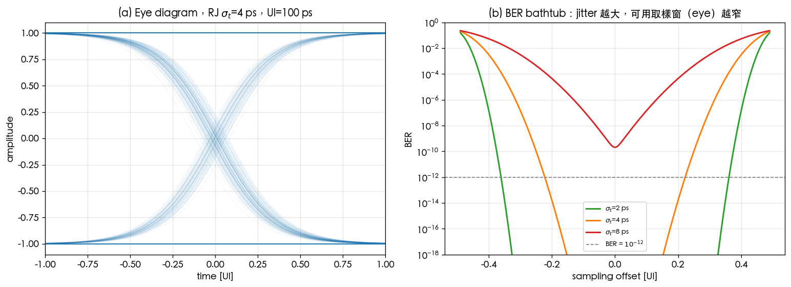
題目:UI = 35.7 ps(28 Gbps)、RJ-only σt=2 ps。問在 eye 中央(sampling offset t=0)的 BER?
又若 σt 惡化到 4 ps,BER 變多少?
逐步解
第 1 步,RJ-only BER bathtub(規範第 10.2 節 SerDes BER):
BER(t)=21[Q(σtUI/2−t)+Q(σtUI/2+t)],Q(x)=21erfc(x/2)。
第 2 步,eye 中央 t=0 時兩項相同:BER=Q(σtUI/2)。
第 3 步,σt=2 ps:σtUI/2=217.85=8.93。Q(8.93) 是極小數(高斯尾),
≈2×10⁻¹⁹。σt=4 ps:417.85=4.46,Q(4.46)≈4×10⁻⁶。
結果:σt=2 ps → BER ≈2×10⁻¹⁹;σt=4 ps → BER ≈4×10⁻⁶。
jitter 加倍 → BER 惡化 13 個數量級(高斯尾對 σ 極度敏感)。
Dimension check:Q 的引數 σtUI/2=[s][s] 無因次 ✓;BER 無因次(機率)✓。
手感:這就是為什麼 SerDes 規格用 σt(rms)但 BER 看的是 σ 的「倍數」(Q 函數);
省一點 jitter 能換來 BER 巨幅改善。對照圖:
Python 驗證
import numpy as np
from simulations.common.serdes_utils import ber_bathtub
ui = 1/28e9
for st in [2e-12, 4e-12]:
ber = ber_bathtub(np.array([0.0]), sigma_t=st, ui=ui)[0]
print(st*1e12, "ps -> BER =", f"{ber:.2e}")
自我檢查表
做完上面 15 題後,遮住答案問自己——每一項都該能在腦中「秒答方向」:
A 級(換算反射)
B 級(ISF → phase noise)
C 級(jitter 積分)
D 級(設計反推)
誠實標記
- 例 C3 的 period jitter 前置常數標了
TODO: manual verification needed(與單邊/雙邊譜慣例有關)。
- 例 D3 的 ring Γrms∝N−3/2([P2] Eq.(16), p.794;v7 已重核:根號只蓋常數;正文 4/N1.5@η=0.75
與 App.B Eq.(55) 三重驗證;v3 曾誤讀為 N−3/4)。「14.3 dB」是 N=5→15 時 Γrms2 比值
(15/5)−3=1/27 換算成 dB 的正確結果(10log10(1/27)=−14.3 dB),但仍僅為孤立因子示意,
非真實設計增益(toy scaling,非 transistor-level;見 D3 警語段的 FOM N-independence)。
延伸閱讀