β: This English translation is in beta — the Traditional-Chinese original is the authoritative version.

Worked Examples

This page is the hands-on worked-example bank for ISF / phase noise / jitter. The theory pages show where the formulas come from; here you learn to plug in the numbers, compute all the way through, check the units, and verify with one line of Python. All formulas are carried over verbatim from [the AUTHORING_SPEC authoritative formula table]; numbers follow numerical_feeling and the spec Section 8 canonical values ($q_{max}=1$ pC, $\Gamma_{rms}=0.5$, $f_0=5$ GHz, $\mathcal{L}(1\text{MHz})=-100$ dBc/Hz).

How to use this page: cover the step-by-step solution, work each problem yourself, then check. The core skill of an analog designer is order-of-magnitude estimation at the whiteboard — seeing "$-100$ dBc/Hz @ 1 MHz, 5 GHz" you should call out "a few hundred fs of jitter" within 30 seconds. The one-line Python at the end of each problem is only for checking, never a substitute for the hand calculation.

Four levels:

• (A) Basic conversions: rad ↔ fs, dBc ↔ linear, phase PSD ↔ $\mathcal{L}$. Drill until they become reflexes.
• (B) ISF → phase noise: Eq.(21)/(23)/(24) algebra — turn $\Gamma_{rms},c_0,q_{max}$ into dBc/Hz.
• (C) jitter integration: integrate $\mathcal{L}(f)$ to get $\sigma_t$; the high-pass kernel of period jitter.
• (D) design back-calculation: how large a $q_{max}/\Gamma_{rms}$ for $-120$ dBc/Hz; how to choose the ring stage count $N$.

Every problem follows a fixed format: Problem → step-by-step solution (with units) → Result → dimension check → one-line Python verification. All Python calls real functions from simulations/common/ (see the spec Section 5 API) and runs as-is.

---

Level A: Basic conversions

This level has only two core relations — memorize them cold:

$$\Delta t=\frac{\Delta\phi}{2\pi f_0},\qquad \mathcal{L}_{\text{linear}}=10^{\mathcal{L}_{\text{dBc/Hz}}/10},\qquad S_\phi=2\,\mathcal{L}_{\text{linear}} .$$

Example A1: phase → time (how many fs is 1 mrad at 5 GHz?)

Problem: $f_0=5$ GHz, $\Delta\phi=1$ mrad; find the timing error $\Delta t$.

Step-by-step solution

Step 1: write the phase→time conversion (spec formula 17, $\Delta t=\Delta\phi/(2\pi f_0)$). The unit of $2\pi f_0$ is rad/s (angular frequency) and $\Delta\phi$ is rad; the quotient is seconds:

$$\Delta t=\frac{\Delta\phi}{2\pi f_0}=\frac{1\times10^{-3}\ \text{rad}}{2\pi\times5\times10^{9}\ \text{rad/s}} .$$

Step 2: evaluate the denominator: $2\pi\times5\times10^{9}=3.1416\times10^{10}$ rad/s.

$$\Delta t=\frac{10^{-3}}{3.1416\times10^{10}}\ \text{s}=3.183\times10^{-14}\ \text{s}=31.8\ \text{fs} .$$

Result: $\Delta t\approx31.8$ fs.

Dimension check: $[\text{rad}]/[\text{rad/s}]=[\text{s}]$ ✓. Intuition anchor: at 5 GHz, "1 mrad ≈ 32 fs"; conversely "1 rad ≈ 31.8 ps" (the very same $31.83$ digits, offset by $10^3$). The period is $T=200$ ps, so 1 mrad is about $1.6\times10^{-4}$ of a period.

Python verification

from simulations.common.noise_utils import phase_to_time_error
print(phase_to_time_error(1e-3, 5e9) * 1e15, "fs")   # -> 31.83 fs

Example A2: dBc/Hz → linear (how much is −100 dBc/Hz?)

Problem: $\mathcal{L}=-100$ dBc/Hz. Convert to linear (power ratio relative to the carrier, per Hz), then recover the phase PSD $S_\phi$.

Step-by-step solution

Step 1: dBc/Hz is the "decibels relative to carrier" unit of $10\log_{10}(\cdot)$; invert by dividing by 10 and raising 10 to that power:

$$\mathcal{L}_{\text{linear}}=10^{\mathcal{L}/10}=10^{-100/10}=10^{-10}\ [\text{1/Hz}] .$$

Step 2: under the small-angle single-tone PM approximation, $\mathcal{L}(f)\approx\tfrac12 S_\phi(f)$ (spec formula 16 and the Section 10.2 "$L\approx\tfrac12 S_\phi$" derivation), so back out the phase PSD:

$$S_\phi=2\,\mathcal{L}_{\text{linear}}=2\times10^{-10}\ \text{rad}^2/\text{Hz} .$$

Result: $\mathcal{L}_{\text{linear}}=10^{-10}$/Hz, $S_\phi=2\times10^{-10}$ rad²/Hz.

Dimension check: dBc/Hz is a dimensionless power ratio per Hz; $\mathcal{L}_{\text{linear}}$ is likewise 1/Hz; after the ×2 it reads as a phase PSD in rad²/Hz (rad² is the unit of phase variance; integrating the variance density over $f$ gives rad²) ✓. Mnemonic: every $-10$ dB = one decade less in linear power; every $-20$ dB = one decade less in voltage/phase amplitude.

Python verification

import numpy as np
from simulations.common.noise_utils import phase_psd_to_l_dbc_per_hz
s_phi = 2 * 10**(-100/10)
print(s_phi, "rad^2/Hz")                       # -> 2e-10
print(phase_psd_to_l_dbc_per_hz(s_phi), "dBc/Hz")  # -> -100.0 (round trip consistent)

Example A3: injected charge → phase step → time (a 1 fC kick)

Problem (canonical Example A): $q_{max}=1$ pC, $\Delta q=1$ fC, $\Gamma=0.5$, $f_0=5$ GHz. Find the phase step $\Delta\phi$ and timing error $\Delta t$ caused by a single impulse.

Step-by-step solution

Step 1: use the operational ISF definition (spec formula 5, $\Delta\phi=\Gamma(\omega_0\tau)\,\Delta q/q_{max}$). $\Gamma$ is dimensionless and $\Delta q/q_{max}$ is dimensionless, so $\Delta\phi$ is a pure number (rad):

$$\Delta\phi=\frac{\Gamma\,\Delta q}{q_{max}}=\frac{0.5\times(1\times10^{-15}\ \text{C})}{1\times10^{-12}\ \text{C}}=5\times10^{-4}\ \text{rad} .$$

In degrees: $5\times10^{-4}\times\dfrac{180}{\pi}\approx0.0286^\circ$.

Step 2: convert to time using the A1 conversion ($f_0=5$ GHz):

$$\Delta t=\frac{5\times10^{-4}}{2\pi\times5\times10^{9}}\ \text{s}\approx1.59\times10^{-14}\ \text{s}=15.9\ \text{fs} .$$

Result: $\Delta\phi=5\times10^{-4}$ rad ($0.0286^\circ$), $\Delta t\approx15.9$ fs.

Dimension check: $\Delta\phi$: $[\text{C}]/[\text{C}]=$ dimensionless ✓; $\Delta t$: $[\text{rad}]/[\text{rad/s}]=[\text{s}]$ ✓. Intuition: 1 fC ≈ 6240 electrons; even at the most sensitive phase it kicks out only ~16 fs. One kick is tiny, but noise kicks continuously and the phase integrator accumulates it (see convolution_derivation).

Python verification

from simulations.common.isf_utils import impulse_to_phase_step
from simulations.common.noise_utils import phase_to_time_error
dphi = impulse_to_phase_step(delta_q=1e-15, gamma_value=0.5, qmax=1e-12)
print(dphi, "rad ->", phase_to_time_error(dphi, 5e9)*1e15, "fs")  # 0.0005 rad -> 15.92 fs

Example A4: phase sensitivity varies with injection phase (a taste of LTV)

Problem: an ideal LC oscillator has ISF $\Gamma(\theta)=-\sin\theta$. With the same $\Delta q=1$ fC and $q_{max}=1$ pC, inject at the zero crossing ($\theta=\pi/2$, maximum waveform slope) and at the peak ($\theta=0$, waveform top), and find $\Delta\phi$ in each case.

Step-by-step solution

Step 1: read off the ISF at both points. Note the phase convention here: with $V\propto\cos\theta$ the peak is at $\theta=0$ and the (falling-edge) zero crossing at $\theta=\pi/2$; the ideal LC has $\Gamma=-\sin\theta$:

$$\Gamma(\theta=\pi/2)=-\sin\tfrac{\pi}{2}=-1,\qquad \Gamma(\theta=0)=-\sin 0=0 .$$

Step 2: substitute each into $\Delta\phi=\Gamma\,\Delta q/q_{max}$ ($\Delta q/q_{max}=10^{-15}/10^{-12}=10^{-3}$):

$$\Delta\phi_{\text{ZC}}=(-1)(10^{-3})=-1\times10^{-3}\ \text{rad},\qquad \Delta\phi_{\text{peak}}=(0)(10^{-3})=0\ \text{rad}.$$

Result: injection at the zero crossing → $-1$ mrad (maximum phase effect); injection at the peak → 0 rad (pure amplitude change, no phase change).

Dimension check: both are $[\,]\cdot[\text{C}]/[\text{C}]=$ rad ✓. This is the essence of LTV (linear time-variant) behavior: the effect of the same impulse depends on which phase of the waveform it kicks. $\Gamma=0$ at the peak because the perturbation there is purely radial (amplitude) with no tangential (phase) component, and amplitude is pulled back by the restoring mechanism. See impulse_to_phase_shift.

Python verification

import numpy as np
from simulations.common.isf_utils import gamma_lc_ideal, impulse_to_phase_step
for name, th in [("ZC", np.pi/2), ("peak", 0.0)]:
    g = gamma_lc_ideal(th)                       # = -sin(theta)
    print(name, impulse_to_phase_step(1e-15, g, 1e-12), "rad")
# ZC -0.001 rad ; peak 0.0 rad

---

Level B: ISF → phase noise (algebra)

This level repeatedly uses three signature formulas (all [P1], carried verbatim from spec Section 3):

• White noise 1/f² [P1] Eq.(21), p.185: $\mathcal{L}=10\log_{10}\!\big(\frac{\Gamma_{rms}^2}{q_{max}^2}\cdot\frac{\overline{i_n^2}/\Delta f}{4\Delta\omega^2}\big)$
• flicker 1/f³ [P1] Eq.(23), p.185: contains the $c_0^2$ and $\omega_{1/f}/\Delta\omega$ factors.
• 1/f³ corner [P1] Eq.(24), p.185: $\Delta\omega_{1/f^3}=\omega_{1/f}\,c_0^2/(2\Gamma_{rms}^2)$.

Reminder: the denominator of Eq.(21) is $4\Delta\omega^2$ (SSB bookkeeping convention). A clean time-domain derivation gives $2\Delta\omega^2$; the factor of 2 is a well-known minor dispute in the literature and does not affect the $\Gamma_{rms}^2/q_{max}^2$ scaling or the $-20$ dB/dec slope. See white_noise_to_phase_noise. This page uses the $4\Delta\omega^2$ of the original [P1] expression throughout.

Example B1: white noise → L (canonical Example B, computed to the last digit)

Problem: $f_0=5$ GHz, $\Delta f=1$ MHz offset, $q_{max}=1$ pC, $\Gamma_{rms}=0.5$, white noise $\overline{i_n^2}/\Delta f=S_i=10^{-24}$ A²/Hz. Use Eq.(21) to find $\mathcal{L}(1\text{MHz})$.

Step-by-step solution

Step 1: convert the offset frequency to angular frequency: $\Delta\omega=2\pi\Delta f=2\pi\times10^{6}=6.283\times10^{6}$ rad/s, $\Delta\omega^2=3.948\times10^{13}\ (\text{rad/s})^2$.

Step 2: evaluate the bracket of Eq.(21) (separate the dimensionless part from the part carrying units first):

$$\frac{\Gamma_{rms}^2}{q_{max}^2}=\frac{0.25}{(10^{-12})^2}=0.25\times10^{24}=2.5\times10^{23}\ \text{C}^{-2} .$$ $$\frac{S_i}{4\Delta\omega^2}=\frac{10^{-24}}{4\times3.948\times10^{13}}=\frac{10^{-24}}{1.579\times10^{14}}=6.333\times10^{-39}\ \text{A}^2/\text{Hz}\cdot\text{s}^2 .$$

Step 3: multiply (units checked below):

$$2.5\times10^{23}\times6.333\times10^{-39}=1.583\times10^{-15} .$$

Step 4: take $10\log_{10}$:

$$\mathcal{L}=10\log_{10}(1.583\times10^{-15})=-148.0\ \text{dBc/Hz} .$$

Result: $\mathcal{L}(1\text{MHz})=-148.0$ dBc/Hz.

Dimension check: the bracket must be dimensionless (argument of a log). $[\text{C}^{-2}]\cdot[\text{A}^2\,\text{Hz}^{-1}\,\text{s}^2]$; with $\text{A}=\text{C/s}$ ⇒ $\text{A}^2=\text{C}^2/\text{s}^2$, $\text{Hz}^{-1}=\text{s}$, collect $\text{C}^{-2}\cdot(\text{C}^2/\text{s}^2)\cdot\text{s}\cdot\text{s}^2=\text{C}^{-2}\cdot\text{C}^2\cdot\text{s}^{-2}\cdot\text{s}^{3}=\text{s}$. One $1/\text{s}$ is still missing — it comes from the per-Hz nature of a PSD: the result is "relative power per Hz", so the argument is really 1/Hz, and after the log it is dBc/Hz ✓. (This is exactly why the units are easy to misread; just remember "the final answer is dBc/Hz".)

Intuition: this is the floor set by a single ideal white-noise source. Real circuits have multiple noise sources, cyclostationarity, and flicker; measurements come in tens of dB higher.

Python verification

import numpy as np
Grms, qmax, Si = 0.5, 1e-12, 1e-24
dw = 2*np.pi*1e6
L = 10*np.log10((Grms**2/qmax**2) * (Si/(4*dw**2)))
print(round(L, 2), "dBc/Hz")    # -> -148.0

Example B2: use Parseval to get $\Gamma_{rms}$ from $c_n$, then compute L

Problem: the ideal-LC ISF is purely $\Gamma(\theta)=-\sin\theta$, i.e. only the first harmonic $c_1=1$ and all other $c_n=0$. (a) Use Parseval (Eq.(20)) to find $\Gamma_{rms}$; (b) with $q_{max}=1$ pC, $S_i=10^{-24}$, $\Delta f=1$ MHz, find L.

Step-by-step solution

Step 1 (a): Parseval ([P1] Eq.(20)): $\sum_n c_n^2=2\Gamma_{rms}^2$. Here $\sum_n c_n^2=c_1^2=1$, so

$$2\Gamma_{rms}^2=1\ \Rightarrow\ \Gamma_{rms}=\frac{1}{\sqrt2}\approx0.707 .$$

(Direct check: $\Gamma_{rms}^2=\frac{1}{2\pi}\int_0^{2\pi}\sin^2\theta\,d\theta=\tfrac12$, which also gives $\Gamma_{rms}=1/\sqrt2$ ✓.)

Step 2 (b): substitute into Eq.(21) with $\Gamma_{rms}^2=0.5$:

$$\mathcal{L}=10\log_{10}\!\left(\frac{0.5}{(10^{-12})^2}\cdot\frac{10^{-24}}{4\times3.948\times10^{13}}\right) =10\log_{10}(3.166\times10^{-15})=-145.0\ \text{dBc/Hz} .$$

Result: $\Gamma_{rms}=0.707$; $\mathcal{L}(1\text{MHz})=-145.0$ dBc/Hz.

Dimension check: $\Gamma_{rms}$ is dimensionless (the $c_n$ are dimensionless) ✓; L same as Example B1, dBc/Hz ✓. Note $\Gamma_{rms}=0.707$ is larger than the canonical $0.5$, so L comes out about $3$ dB above B1 ($10\log_{10}(0.5/0.25)=3$ dB) — consistent.

Python verification

import numpy as np
from simulations.common.isf_utils import gamma_lc_ideal, gamma_rms
theta = np.linspace(0, 2*np.pi, 100000, endpoint=False)
Grms = gamma_rms(theta, gamma_lc_ideal(theta))
print("Grms =", round(Grms, 4))                       # -> 0.7071
L = 10*np.log10((Grms**2/(1e-12)**2)*(1e-24/(4*(2*np.pi*1e6)**2)))
print(round(L, 2), "dBc/Hz")                           # -> -145.0

Example B3: symmetry and 1/f³ (the role of $c_0$)

Problem: two oscillators with identical white noise and $q_{max}$, $\omega_{1/f}=2\pi\times1$ MHz. A has a fully symmetric waveform ($c_0=0$); B is slightly asymmetric ($c_0=0.2$, $c_1=1$). Which one shows close-in 1/f³ upconversion? What is each 1/f³ contribution at $\Delta f=10$ kHz?

Step-by-step solution

Step 1: look at Eq.(23) — phase noise in the 1/f³ region is proportional to $c_0^2$.

$$\mathcal{L}_{1/f^3}=10\log_{10}\!\left(\frac{c_0^2}{q_{max}^2}\cdot\frac{S_i}{8\Delta\omega^2}\cdot\frac{\omega_{1/f}}{\Delta\omega}\right) .$$

Step 2, for A: $c_0=0\Rightarrow$ the bracket $=0\Rightarrow \mathcal{L}_{1/f^3}\to-\infty$ dBc/Hz (no flicker upconversion; the 1/f³ region is fully suppressed). In practice it never truly reaches $-\infty$ (other mechanisms take over), but it can sit far below B.

Step 3, for B: $c_0=0.2$, a finite value. Use Eq.(24) to compare the two 1/f³ corners:

$$\Delta\omega_{1/f^3}=\omega_{1/f}\cdot\frac{c_0^2}{2\Gamma_{rms}^2} .$$

For B, $\sum c_n^2=c_0^2+c_1^2=0.04+1=1.04\Rightarrow\Gamma_{rms}^2=0.52$, so

$$\Delta\omega_{1/f^3,B}=\omega_{1/f}\cdot\frac{0.04}{2\times0.52}=\omega_{1/f}\times0.0385 .$$

That is, B's 1/f³ corner sits at $\approx0.0385\,\omega_{1/f}=2\pi\times38.5$ kHz. For A, the corner $\to0$.

Result: A (symmetric, $c_0=0$) has no 1/f³ upconversion; B ($c_0=0.2$) does, with a corner near $38.5$ kHz. Design rule: suppress $c_0$ through waveform symmetry and the 1/f³ corner can be pushed far below the device $\omega_{1/f}$.

Dimension check: in Eq.(24), $c_0^2/\Gamma_{rms}^2$ is dimensionless; multiplying by $\omega_{1/f}$ (rad/s) gives rad/s ✓.

Python verification

import numpy as np
w_1f = 2*np.pi*1e6
for name, c0, c1 in [("A", 0.0, 1.0), ("B", 0.2, 1.0)]:
    Grms2 = 0.5*(c0**2 + c1**2)          # Parseval: sum cn^2 = 2 Grms^2
    corner = w_1f * c0**2/(2*Grms2)
    print(name, "1/f^3 corner =", corner/(2*np.pi)*1e-3, "kHz")
# A 0.0 kHz ; B 38.46 kHz

Example B4: white-noise floor and the −20 dB/dec slope vs offset

Problem: reuse the B1 oscillator ($\mathcal{L}(1\text{MHz})=-148$ dBc/Hz, 1/f² region). What is L at $\Delta f=10$ MHz? (I.e. push the offset out by 10×.)

Step-by-step solution

Step 1: in Eq.(21), $\mathcal{L}\propto1/\Delta\omega^2$; after the log this is $-20\log_{10}\Delta\omega+$const, i.e. every 10× in offset drops L by 20 dB ($-20$ dB/decade).

Step 2: $\Delta f$ goes from 1 MHz → 10 MHz (×10):

$$\mathcal{L}(10\text{MHz})=\mathcal{L}(1\text{MHz})-20\log_{10}(10)=-148-20=-168\ \text{dBc/Hz} .$$

Result: $\mathcal{L}(10\text{MHz})=-168$ dBc/Hz.

Dimension check: the argument of $-20\log_{10}(\Delta f_2/\Delta f_1)$ is dimensionless (a frequency ratio) ✓; the result is a dB difference, and adding it to dBc/Hz still gives dBc/Hz ✓. Intuition: "20 dB per decade" in the 1/f² region is the most-used visual slope on a phase-noise plot; compare $-30$ dB/dec in the 1/f³ region.

Python verification

import numpy as np
Grms, qmax, Si = 0.5, 1e-12, 1e-24
def L(df): return 10*np.log10((Grms**2/qmax**2)*(Si/(4*(2*np.pi*df)**2)))
print(round(L(1e6),2), round(L(10e6),2), "dBc/Hz",
      "slope =", round(L(10e6)-L(1e6),1), "dB/dec")   # -148.0 -168.0 ; -20.0

---

Level C: jitter integration

Core idea: phase noise is a frequency-domain density, jitter is a time-domain rms; they connect via "integrate + square root + $\div(2\pi f_0)$" (spec formulas 18, 19):

$$\sigma_\phi^2=\int_{f_1}^{f_2}S_\phi(f)\,df,\qquad \sigma_t=\frac{\sigma_\phi}{2\pi f_0} .$$

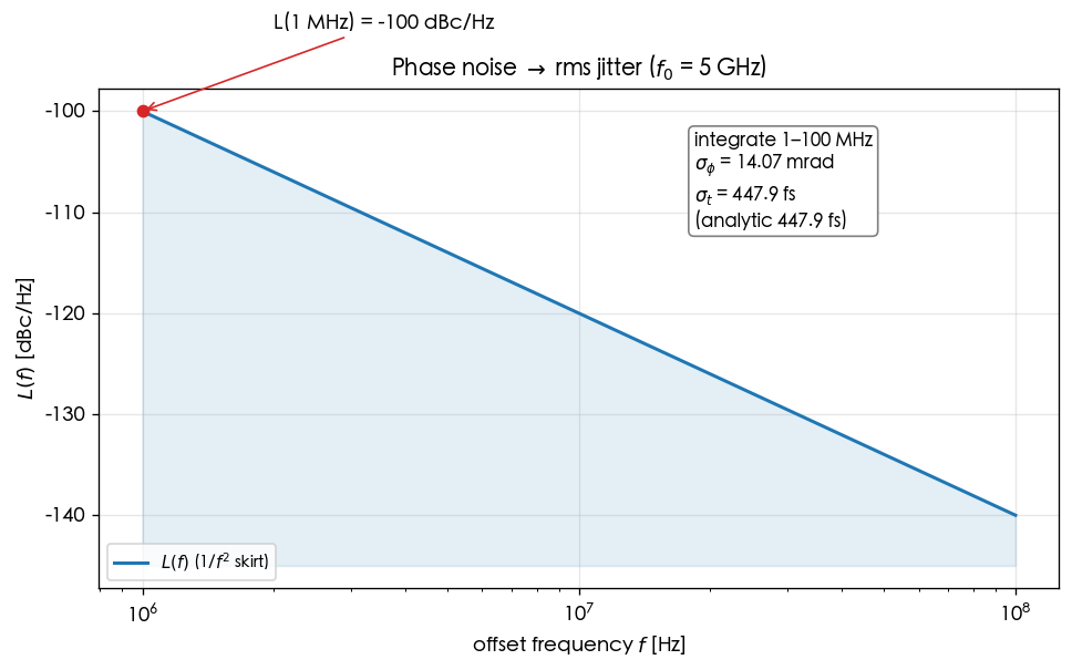
Example C1: L(f) → rms jitter (canonical Example C, 1/f² integration)

Problem: $\mathcal{L}(1\text{MHz})=-100$ dBc/Hz, 1/f² slope, integrate from $f_1=1$ MHz to $f_2=100$ MHz, $f_0=5$ GHz. Find $\sigma_\phi$ and $\sigma_t$.

Step-by-step solution

Step 1: convert the datasheet point to a phase PSD (using A2): $S_\phi(f_{ref})=2\times10^{-10}$ rad²/Hz, $f_{ref}=1$ MHz.

Step 2: write the 1/f² shape (anchored at $f_{ref}$):

$$S_\phi(f)=S_\phi(f_{ref})\left(\frac{f_{ref}}{f}\right)^2=2\times10^{-10}\,(10^6)^2\,\frac1{f^2} .$$

Step 3: integrate ($\int f^{-2}df=-1/f$):

$$\sigma_\phi^2=2\times10^{-10}(10^6)^2\!\int_{10^6}^{10^8}\!\frac{df}{f^2} =2\times10^{2}\left(\frac1{10^6}-\frac1{10^8}\right)=200\times9.9\times10^{-7}=1.98\times10^{-4}\ \text{rad}^2 .$$

So $\sigma_\phi=\sqrt{1.98\times10^{-4}}=1.407\times10^{-2}$ rad $=14.07$ mrad.

Step 4: convert to rms jitter ($f_0=5$ GHz):

$$\sigma_t=\frac{\sigma_\phi}{2\pi f_0}=\frac{1.407\times10^{-2}}{2\pi\times5\times10^{9}}\approx4.48\times10^{-13}\ \text{s}=447.9\ \text{fs} .$$

Result: $\sigma_\phi=14.07$ mrad, $\sigma_t=447.9$ fs.

Dimension check: $\sigma_\phi^2$: $[\text{rad}^2/\text{Hz}]\cdot[\text{Hz}]=\text{rad}^2$ ✓; $\sigma_t$: $[\text{rad}]/[\text{rad/s}]=[\text{s}]$ ✓. Intuition: the 1/f² integral is dominated by the lower limit $f_1$ ($1/f_1\gg1/f_2$) — where you start integrating matters most. With $-120$ dBc/Hz @ 1 MHz instead (20 dB better = 1/100 the power, 1/10 the amplitude), the jitter shrinks to ~45 fs.

Python verification

import numpy as np
from simulations.common.noise_utils import leeson_one_over_f2, integrate_rms_jitter
f = np.logspace(6, 8, 4000)                              # 1 MHz -> 100 MHz
L = leeson_one_over_f2(f, L_ref_dbc=-100, f_ref=1e6)     # 1/f^2 skirt
sigma_t, sigma_phi = integrate_rms_jitter(f, L, f0=5e9, fmin=1e6, fmax=100e6)
print(round(sigma_phi*1e3,2), "mrad ;", round(sigma_t*1e15,1), "fs")  # 14.07 mrad ; 447.9 fs

Example C2: lower-limit dominance — what if the lower limit moves?

Problem: same spectrum as C1 ($-100$ dBc/Hz @ 1 MHz, 1/f², $f_0=5$ GHz), but integrate from $f_1=100$ kHz to 100 MHz. Estimate $\sigma_t$ and compare with C1.

Step-by-step solution

Step 1: for 1/f², $\sigma_\phi^2\propto(1/f_1-1/f_2)\approx1/f_1$ (lower-limit dominated). The lower limit moves from $10^6$ to $10^5$ (10× smaller), so $1/f_1$ is 10× larger:

$$\sigma_\phi^2\approx2\times10^{2}\left(\frac1{10^5}-\frac1{10^8}\right)=200\times(10^{-5}-10^{-8})\approx2.0\times10^{-3}\ \text{rad}^2 .$$

Step 2: $\sigma_\phi=\sqrt{2.0\times10^{-3}}=4.47\times10^{-2}$ rad $=44.7$ mrad (about $\sqrt{10}\approx3.16$× C1).

Step 3: $\sigma_t=\dfrac{4.47\times10^{-2}}{2\pi\times5\times10^{9}}\approx1.42\times10^{-12}$ s $=1.42$ ps.

Result: $\sigma_t\approx1.42$ ps (C1 was 448 fs). Lowering the limit by 10× → jitter grows by about $\sqrt{10}\approx3.16$×.

Dimension check: same as C1 ✓. Intuition: this is why an "rms jitter" number is only meaningful with its integration band attached; the instrument's lower limit (or the PLL loop bandwidth) determines how much accumulated jitter you get to see.

Python verification

import numpy as np
from simulations.common.noise_utils import leeson_one_over_f2, integrate_rms_jitter
f = np.logspace(5, 8, 6000)                              # 100 kHz -> 100 MHz
L = leeson_one_over_f2(f, L_ref_dbc=-100, f_ref=1e6)
sigma_t, sigma_phi = integrate_rms_jitter(f, L, f0=5e9, fmin=1e5, fmax=100e6)
print(round(sigma_phi*1e3,1), "mrad ;", round(sigma_t*1e12,2), "ps")  # ~44.7 mrad ; ~1.42 ps

Example C3: the high-pass kernel of period jitter

Problem: period jitter (the deviation of a single period, $T_k-T$) is the first difference of phase. Using the spec Section 10.2 kernel $\lvert1-e^{-j2\pi fT}\rvert^2$, estimate the period jitter $\sigma_T$ for the C1 spectrum ($-100$ dBc/Hz @ 1 MHz, 1/f², $f_0=5$ GHz, $T=200$ ps).

Step-by-step solution

Step 1: write the period-jitter formula (spec Section 10.2 period/cycle-to-cycle kernel):

$$\sigma_T^2=\frac1{(2\pi f_0)^2}\int_0^{\infty}S_\phi(f)\,\lvert1-e^{-j2\pi fT}\rvert^2\,df .$$

Step 2: understand what the kernel does: $\lvert1-e^{-j2\pi fT}\rvert^2=2(1-\cos2\pi fT)=4\sin^2(\pi fT)$ is high-pass — low frequencies ($fT\ll1$) are suppressed ($\propto f^2$), so period jitter is not dominated by the low-frequency 1/f² lower limit (opposite to the accumulated jitter of C1/C2). This is why period jitter is usually much smaller than the "accumulated jitter" of the same spectrum.

Step 3: numerical integration (not feasible by hand — hand it to the computer; constants aligned with the spec kernel). See the Python below: $\sigma_T\approx27.6$ fs.

Result: $\sigma_T\approx27.6$ fs (versus the C1 accumulated $\sigma_t=448$ fs — more than an order of magnitude smaller).

Dimension check: the kernel $\lvert1-e^{-j2\pi fT}\rvert^2$ is dimensionless; $\int S_\phi\,(\text{kernel})\,df$ gives rad²; dividing by the $(\text{rad/s})^2$ of $(2\pi f_0)^2$… note the order: first rad², then dividing by $(2\pi f_0)^2$ gives s², and the square root gives s ✓. Resolved (v5): the exact prefactor for period/cycle-to-cycle jitter has been derived from first principles + Monte-Carlo verified in jitter_kernels (under the single-sided $S_\phi$ convention the kernel is $4\sin^2$ with prefactor $1/\omega_0^2$; the 27.6 fs here is the band-limited version of that page's closed-form 28.28 fs) Cross-check against standard references; here we use the kernel given in spec Section 10.2, and the number is for order-of-magnitude feel only.

Python verification

import numpy as np
T, f0, fref, Lref = 1/5e9, 5e9, 1e6, -100
f = np.logspace(3, 10, 2_000_000)                        # wide band: the high-pass kernel suppresses low f
S_phi = 2 * 10**((Lref + 20*np.log10(fref/f))/10)        # 1/f^2 phase PSD
kernel = np.abs(1 - np.exp(-1j*2*np.pi*f*T))**2          # first-difference high-pass kernel
trapz = getattr(np, "trapezoid", np.trapz)
sigma_T = np.sqrt(trapz(S_phi*kernel, f)) / (2*np.pi*f0)
print(round(sigma_T*1e15, 1), "fs")                      # ~27.6 fs

Example C4: ring accumulated jitter $\sigma_{\Delta t}=\kappa\sqrt{\Delta t}$

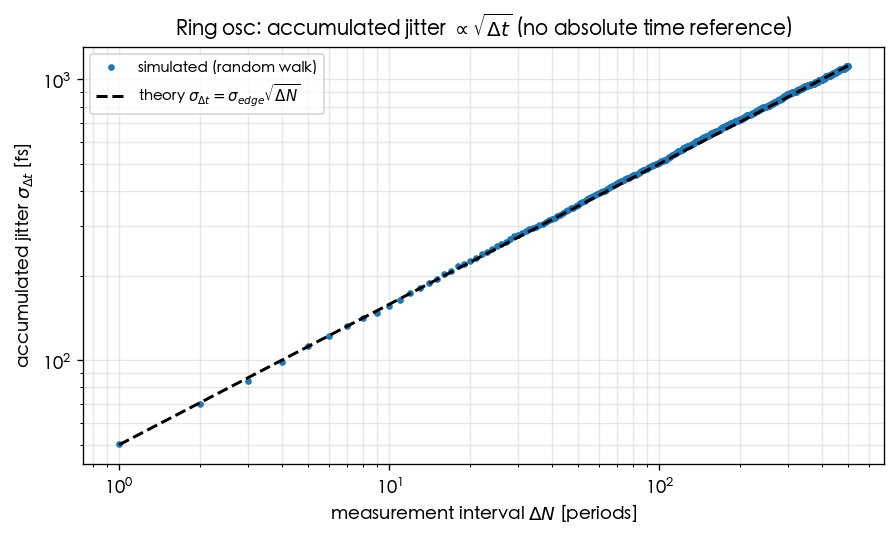
Problem ([P2] Eq.(8)): a ring has jitter proportionality constant $\kappa=1\times10^{-8}\ \sqrt{\text{s}}$ (toy value). Find the accumulated rms jitter for measurement intervals $\Delta t=1\ \mu$s and $\Delta t=1$ ms.

Step-by-step solution

Step 1: the random-walk law ([P2] Eq.(8), the signature of an oscillator with no absolute time reference): $\sigma_{\Delta t}=\kappa\sqrt{\Delta t}$.

Step 2: $\Delta t=10^{-6}$ s:

$$\sigma_{\Delta t}=10^{-8}\sqrt{10^{-6}}=10^{-8}\times10^{-3}=10^{-11}\ \text{s}=10\ \text{ps} .$$

Step 3: $\Delta t=10^{-3}$ s:

$$\sigma_{\Delta t}=10^{-8}\sqrt{10^{-3}}=10^{-8}\times3.162\times10^{-2}=3.16\times10^{-10}\ \text{s}=316\ \text{ps} .$$

Result: 1 μs → 10 ps; 1 ms → 316 ps. Interval ×1000, jitter ×$\sqrt{1000}\approx31.6$.

Dimension check: $\kappa$ has units of $\sqrt{\text{s}}$, $\sqrt{\Delta t}$ is $\sqrt{\text{s}}$, and their product is s ✓ (which is also why $\kappa$ carries that odd unit). Intuition: the phase of a ring (no high-Q tank) is a pure random walk — the longer you wait, the larger the error, and it never converges. This is exactly the time-domain picture of why rings are noisier than LC. Companion figure:

Python verification

import numpy as np
kappa = 1e-8                                  # sqrt(s)
for dt in [1e-6, 1e-3]:
    print(dt, "s ->", kappa*np.sqrt(dt)*1e12, "ps")
# 1e-06 s -> 10.0 ps ; 0.001 s -> 316.2 ps

---

Level D: design back-calculation

Run the formulas in reverse: given a spec, find the required $q_{max}$, how small $\Gamma_{rms}$ must be, how many stages $N$.

Example D1: how large must $q_{max}$ be for −120 dBc/Hz @ 1 MHz?

Problem: spec $\mathcal{L}(1\text{MHz})=-120$ dBc/Hz, $f_0=5$ GHz. Assume a single white-noise source $S_i=1\times10^{-21}$ A²/Hz (1000× the canonical value, closer to a real node injection) and $\Gamma_{rms}=0.5$. Back-solve the required $q_{max}$.

Step-by-step solution

Step 1: solve Eq.(21) for $q_{max}$. First convert the spec to linear: $\mathcal{L}_{\text{lin}}=10^{-120/10}=10^{-12}$.

$$10^{-12}=\frac{\Gamma_{rms}^2}{q_{max}^2}\cdot\frac{S_i}{4\Delta\omega^2} \ \Rightarrow\ q_{max}^2=\frac{\Gamma_{rms}^2\,S_i}{4\Delta\omega^2\,\mathcal{L}_{\text{lin}}} .$$

Step 2: plug in numbers ($\Delta\omega^2=3.948\times10^{13}$, $\Gamma_{rms}^2=0.25$):

$$q_{max}^2=\frac{0.25\times10^{-21}}{4\times3.948\times10^{13}\times10^{-12}} =\frac{0.25\times10^{-21}}{1.579\times10^{2}}=1.583\times10^{-24}\ \text{C}^2 .$$

Step 3: take the square root: $q_{max}=\sqrt{1.583\times10^{-24}}=1.258\times10^{-12}$ C $=1.26$ pC.

Result: $q_{max}\approx1.26$ pC (i.e. raise the canonical 1 pC by about 26%; at this noise level the spec is met).

Dimension check: $q_{max}^2$: $[\,]\cdot[\text{A}^2\text{Hz}^{-1}]/([\text{rad/s}]^2\cdot[\,])$; with $\text{A}^2\text{Hz}^{-1}=\text{C}^2\text{s}^{-2}\cdot\text{s}=\text{C}^2\text{s}^{-1}$, dividing by $\text{s}^{-2}$ gives $\text{C}^2\text{s}$, and after absorbing the PSD's per-Hz it is $\text{C}^2$ ✓. Design intuition: $\mathcal{L}\propto1/q_{max}^2$, so doubling $q_{max}$ → 6 dB lower phase noise. Ways to increase $q_{max}=C_{node}V_{max}$: raise the swing $V_{max}$ or the node capacitance/current.

Python verification

import numpy as np
Grms, Si, dw, Llin = 0.5, 1e-21, 2*np.pi*1e6, 10**(-120/10)
qmax = np.sqrt(Grms**2 * Si / (4*dw**2 * Llin))
print(round(qmax*1e12, 3), "pC")     # -> 1.258 pC

Example D2: with $q_{max}$ fixed, how small a $\Gamma_{rms}$ for −120 dBc/Hz?

Problem: same spec and noise as D1 ($-120$ dBc/Hz, $S_i=10^{-21}$, $\Delta f=1$ MHz, $f_0=5$ GHz), but this time $q_{max}=1$ pC is fixed (the swing cannot be raised further). Back-solve the required $\Gamma_{rms}$.

Step-by-step solution

Step 1: solve Eq.(21) for $\Gamma_{rms}$:

$$\Gamma_{rms}^2=\frac{\mathcal{L}_{\text{lin}}\,q_{max}^2\,4\Delta\omega^2}{S_i} =\frac{10^{-12}\times(10^{-12})^2\times4\times3.948\times10^{13}}{10^{-21}} .$$

Step 2: evaluate the numerator term by term: $10^{-12}\times10^{-24}=10^{-36}$; $\times1.579\times10^{14}=1.579\times10^{-22}$. Divide by $10^{-21}$: $\Gamma_{rms}^2=0.1579$.

Step 3: $\Gamma_{rms}=\sqrt{0.1579}=0.397$.

Result: $\Gamma_{rms}\approx0.40$ (the ISF rms must drop from 0.5 to 0.40, about a 20% reduction).

Dimension check: $\Gamma_{rms}^2$ is dimensionless (same argument analysis as B1; all unit-bearing terms cancel) ✓. Design intuition: $\mathcal{L}\propto\Gamma_{rms}^2$, so halving $\Gamma_{rms}$ → 6 dB lower phase noise. Ways to lower $\Gamma_{rms}$: waveform symmetry (suppress $c_0$), schedule noise injection at phases where the ISF is small, more ring stages (see D3). D1 (tune $q_{max}$) and D2 (tune $\Gamma_{rms}$) are two independent knobs toward the same spec.

Python verification

import numpy as np
qmax, Si, dw, Llin = 1e-12, 1e-21, 2*np.pi*1e6, 10**(-120/10)
Grms = np.sqrt(Llin * qmax**2 * 4*dw**2 / Si)
print(round(Grms, 3))     # -> 0.397

Example D3: choosing the ring stage count $N$ (frequency vs ISF)

Problem: build an $f_0=5$ GHz single-ended ring. (a) With per-stage delay $\tau_D=20$ ps, how many stages $N$? (b) Going from $N=5$ to $N=15$ stages (adjusting $\tau_D$ to hold $f_0$), use $\Gamma_{rms}\propto N^{-3/2}$ to estimate the phase-noise change in dB (looking at the $\Gamma_{rms}$ factor only).

Step-by-step solution

Step 1 (a): ring frequency ([P2] Eq.(15)): $f_0=\dfrac1{2N\tau_D}\Rightarrow N=\dfrac1{2f_0\tau_D}$.

$$N=\frac1{2\times5\times10^{9}\times20\times10^{-12}}=\frac1{0.2}=5 .$$

Step 2 (b): $\Gamma_{rms}\propto N^{-3/2}$ ([P2] Eq.(16), p.794, re-verified in v7: the square root covers only the constant; the body text's $4/N^{1.5}$@$\eta=0.75$ and App.B Eq.(55) triple-confirm this. v3 had misread it as $N^{-3/4}$; scaling-level statement). Ratio:

$$\frac{\Gamma_{rms}(15)}{\Gamma_{rms}(5)}=\left(\frac{15}{5}\right)^{-3/2}=3^{-1.5}=0.1925 .$$

Step 3: phase noise $\propto\Gamma_{rms}^2$, so the change (dB):

$$\Delta\mathcal{L}=10\log_{10}\!\big(0.1925^2\big)=10\log_{10}(0.0370)=-14.3\ \text{dB} .$$

Result: (a) $N=5$ stages. (b) Looking at the $\Gamma_{rms}$ term alone, going from $N=5$ to 15 lowers phase noise by about 14.3 dB.

Dimension check: $N=1/(2f_0\tau_D)$: $1/([\text{Hz}][\text{s}])=1/([\text{s}^{-1}][\text{s}])=$ dimensionless ✓ ($N$ must be an integer; here it comes out exact). $\Delta\mathcal{L}$: the argument of $10\log_{10}$ is a dimensionless ratio ✓.

Important caveat: the above isolates $\Gamma_{rms}$ only. The full [P2] conclusion is — at fixed $f_0$ and total power $P$, the phase noise / jitter of a single-ended ring is nearly independent of $N$ (see the FOM in [P2] Eq.(23), p.796, verified). Increasing $N$ does lower $\Gamma_{rms}$, but the noise sources multiply and the per-stage swing/power allocation changes, and these cancel. So the "14.3 dB" of D3(b) is a single-factor teaching illustration, not a gain a real design gets for free. See lc_vs_ring and lab_03. This is pedagogical toy scaling, not transistor-level.

Python verification

import numpy as np
f0, tauD = 5e9, 20e-12
N = 1/(2*f0*tauD)
print("N =", N)                                   # -> 5.0
ratio = (15/5)**-1.5                               # Grms scaling
print("dPN =", round(10*np.log10(ratio**2), 1), "dB")   # -> -14.3 dB (Grms factor only)

Example D4: back-solving phase noise from a jitter spec (SerDes link)

Problem: a 5 GHz clock requires integrated rms jitter $\sigma_t\le100$ fs (integrated 1 MHz→100 MHz, 1/f² spectrum). Back-solve how low $\mathcal{L}$ must be at 1 MHz.

Step-by-step solution

Step 1: C1 already established the mapping — for the same integration band and 1/f² shape, $\sigma_t\propto\sqrt{\mathcal{L}_{\text{lin}}(f_{ref})}$ (since $\sigma_\phi^2\propto S_\phi(f_{ref})\propto\mathcal{L}_{\text{lin}}$, then take the square root). C1 baseline: $\mathcal{L}=-100$ dBc/Hz → $\sigma_t=447.9$ fs.

Step 2: getting from 447.9 fs down to 100 fs is a factor of $447.9/100=4.479$. Jitter is a voltage/amplitude-like quantity, so reducing it by $k$ corresponds to reducing phase-noise power by $k^2$:

$$\Delta\mathcal{L}=-20\log_{10}(4.479)=-13.0\ \text{dB} .$$

Step 3: required level: $-100-13.0=-113.0$ dBc/Hz @ 1 MHz.

Result: $\mathcal{L}(1\text{MHz})\approx-113$ dBc/Hz is needed (1/f², integrated 1→100 MHz) to reach $\sigma_t\le100$ fs.

Dimension check: the argument of $-20\log_{10}(\text{ratio})$ is dimensionless ✓; the dB difference added to dBc/Hz is still dBc/Hz ✓. SerDes link: 100 fs RJ in a high-speed SerDes (e.g. UI = 1/(28 Gbps) ≈ 35.7 ps) directly determines eye closure and BER; see lab_12 and serdes_clocking_connection.

Python verification

import numpy as np
from simulations.common.noise_utils import leeson_one_over_f2, integrate_rms_jitter
target_fs = 100.0
# measure sigma_t from the -100 baseline, then back-solve the required dBc/Hz via the square law
f = np.logspace(6, 8, 4000)
L0 = leeson_one_over_f2(f, L_ref_dbc=-100, f_ref=1e6)
st0, _ = integrate_rms_jitter(f, L0, f0=5e9, fmin=1e6, fmax=100e6)
L_req = -100 - 20*np.log10((st0*1e15)/target_fs)
print(round(L_req, 1), "dBc/Hz @ 1 MHz")     # -> -113.0 dBc/Hz

Example D5: SerDes BER bathtub (how RJ hits the eye)

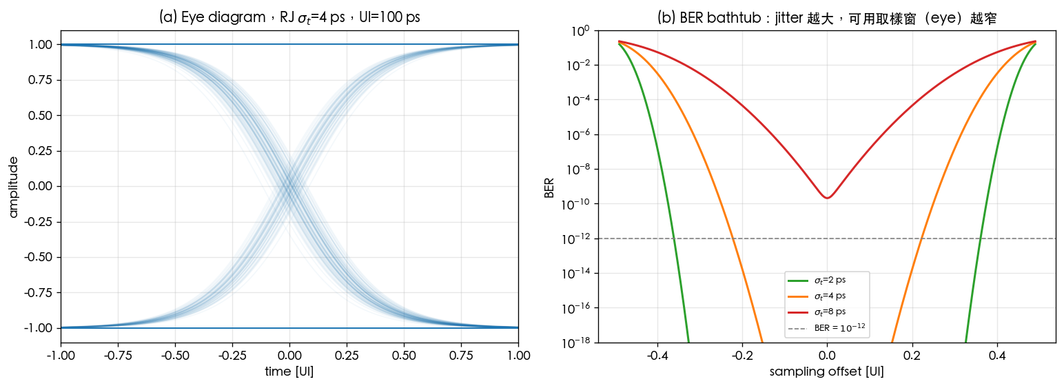
Problem: UI = 35.7 ps (28 Gbps), RJ-only $\sigma_t=2$ ps. What is the BER at eye center (sampling offset $t=0$)? And if $\sigma_t$ degrades to 4 ps, what does the BER become?

Step-by-step solution

Step 1: RJ-only BER bathtub (spec Section 10.2 SerDes BER): $\text{BER}(t)=\tfrac12[Q(\tfrac{UI/2-t}{\sigma_t})+Q(\tfrac{UI/2+t}{\sigma_t})]$, $Q(x)=\tfrac12\mathrm{erfc}(x/\sqrt2)$.

Step 2: at eye center $t=0$ the two terms are equal: $\text{BER}=Q\!\big(\tfrac{UI/2}{\sigma_t}\big)$.

Step 3: for $\sigma_t=2$ ps: $\dfrac{UI/2}{\sigma_t}=\dfrac{17.85}{2}=8.93$. $Q(8.93)$ is a vanishingly small number (Gaussian tail), $\approx2\times10^{-19}$. For $\sigma_t=4$ ps: $\dfrac{17.85}{4}=4.46$, $Q(4.46)\approx4\times10^{-6}$.

Result: $\sigma_t=2$ ps → BER $\approx2\times10^{-19}$; $\sigma_t=4$ ps → BER $\approx4\times10^{-6}$. Doubling the jitter → BER degrades by 13 orders of magnitude (the Gaussian tail is extremely sensitive to $\sigma$).

Dimension check: the argument of $Q$, $\dfrac{UI/2}{\sigma_t}=\dfrac{[\text{s}]}{[\text{s}]}$, is dimensionless ✓; BER is dimensionless (a probability) ✓. Intuition: this is why SerDes specs quote $\sigma_t$ (rms) while BER depends on the multiple of $\sigma$ (the $Q$ function); a modest jitter saving buys a huge BER improvement. Companion figure:

Python verification

import numpy as np
from simulations.common.serdes_utils import ber_bathtub
ui = 1/28e9
for st in [2e-12, 4e-12]:
    ber = ber_bathtub(np.array([0.0]), sigma_t=st, ui=ui)[0]
    print(st*1e12, "ps -> BER =", f"{ber:.2e}")
# 2.0 ps -> BER ~ 2e-19 ; 4.0 ps -> BER ~ 4e-06

---

Self-check list

After finishing the 15 problems above, cover the answers and quiz yourself — every item should get an instant "direction" answer in your head:

Level A (conversion reflexes)

• Given a phase error (rad), immediately convert to time (s) via $\div(2\pi f_0)$ and run the $[\text{rad}]/[\text{rad/s}]=[\text{s}]$ check.
• Remember "at 5 GHz: 1 mrad ≈ 32 fs, 1 rad ≈ 31.8 ps".
• dBc/Hz → linear ($10^{\mathcal{L}/10}$) → phase PSD ($\times2$) in one breath.
• Understand why $\Delta\phi=\Gamma\,\Delta q/q_{max}$ is dimensionless, and that the ISF varies with injection phase (LTV).

Level B (ISF → phase noise)

• Can write Eq.(21) from memory and plug in numbers to get dBc/Hz; know the denominator is $4\Delta\omega^2$ (SSB convention).
• Can use Parseval ($\sum c_n^2=2\Gamma_{rms}^2$) to get $\Gamma_{rms}$ from the $c_n$.
• Know that 1/f³ upconversion exists only when $c_0\ne0$, with corner $=\omega_{1/f}c_0^2/(2\Gamma_{rms}^2)$.
• 1/f² is $-20$ dB/dec, 1/f³ is $-30$ dB/dec — read them off a plot by eye.

Level C (jitter integration)

• Can run the full chain dBc/Hz → (integrate) → $\sigma_\phi$ → ($\div2\pi f_0$) → $\sigma_t$.
• Know that 1/f² accumulated jitter is dominated by the lower integration limit; an rms-jitter number must always come with its band.
• Understand that period jitter uses a high-pass kernel and is not dominated by low frequencies; distinguish it from accumulated jitter.
• Remember ring accumulated jitter $\sigma_{\Delta t}=\kappa\sqrt{\Delta t}$ (random walk, never converges).

Level D (design back-calculation)

• Given a dBc/Hz spec, can back-solve $q_{max}$ or $\Gamma_{rms}$ (doubling $q_{max}$ or halving $\Gamma_{rms}$ each gives $-6$ dB).
• Can compute the ring stage count from $f_0=1/(2N\tau_D)$, and remember the caveat "at fixed $f_0,P$, ring PN is nearly independent of $N$".
• Can translate a jitter spec (fs) back into dBc/Hz at 1 MHz (reducing $\sigma_t$ by $k$ ⇒ $\mathcal{L}$ drops by $20\log_{10}k$ dB).
• Know that RJ-limited BER is extremely sensitive to $\sigma_t$ (Gaussian tail); a small jitter improvement → a large BER improvement.

Honesty notes

• The period-jitter prefactor in Example C3 carries TODO: manual verification needed (tied to the single-/double-sided spectrum convention).
• The ring $\Gamma_{rms}\propto N^{-3/2}$ in Example D3 ([P2] Eq.(16), p.794; re-verified in v7: the square root covers only the constant; the body text's $4/N^{1.5}$@$\eta=0.75$ and App.B Eq.(55) triple-confirm this; v3 had misread it as $N^{-3/4}$). The "14.3 dB" is the correct dB conversion of the $\Gamma_{rms}^2$ ratio $(15/5)^{-3}=1/27$ for $N=5\to15$ ($10\log_{10}(1/27)=-14.3$ dB), but it remains a single-factor illustration only, not a real design gain (toy scaling, not transistor-level; see the FOM N-independence caveat in D3).

Further reading

• Conversion-intuition roundup: numerical_feeling
• Full impulse → phase derivation: impulse_to_phase_shift
• White noise → phase noise (Eq.(21) derivation and the factor-of-2): white_noise_to_phase_noise
• Flicker upconversion and symmetry: flicker_noise_upconversion
• Jitter-integration simulation: lab_08
• Design knobs ($q_{max},\Gamma_{rms},N$): lab_09