What Is Oscillator Phase?

β: This English translation is in beta — the Traditional-Chinese original is the authoritative version.

Prerequisites: Notation · Learning path | Next: phase_vs_amplitude_noise

Before talking about the ISF (Impulse Sensitivity Function), one thing must be made absolutely clear: what physical quantity an oscillator's "phase" actually is, how it differs from "amplitude", and why one persists forever while the other is automatically corrected. This page answers that question. It is the foundation of the entire ISF theory — the later derivation from impulse to phase shift stands entirely on the geometric intuition built here.

Physical intuition (conclusion first): draw the oscillator's state in a 2-D plane; in steady state it circles endlessly along a closed loop (the limit cycle). A noise impulse pushes the state point off this loop. The displacement can be split into two directions: along the tangent of the loop = a phase perturbation, perpendicular to the loop, pointing toward the center (radial) = an amplitude perturbation. The oscillator has an "amplitude restoring force" that slowly pulls radial deviations back onto the loop; but no force whatsoever corrects a deviation along the tangent, because the oscillator simply has no absolute reference for "what time it is". So phase errors accumulate, kick after kick — this is the root of phase noise and timing jitter.

Step 1: describing an oscillator with a state trajectory

Any oscillator can be described completely by a few "state variables". The archetypal LC oscillator has two energy-storage elements: a capacitor (stores voltage) and an inductor (stores current), so its state is a 2-D vector

$$\mathbf{z}(t)=\big(x(t),\,y(t)\big),$$

where we may take $x$ = the capacitor voltage (normalized) and $y$ = a quantity proportional to the inductor current (normalized). As time evolves, $\mathbf{z}(t)$ traces a curve in this "state plane", called the state trajectory.

• Physics used: energy sloshes back and forth between the capacitor and the inductor — when the voltage is maximal the current is zero (all energy in the capacitor); when the voltage is zero the current is maximal (all energy in the inductor). This is precisely the picture of a point going around a circle in the $x$–$y$ plane.
• Unit check: both axes are first normalized to be dimensionless (each divided by its maximum swing); the radius $r=\sqrt{x^2+y^2}$ represents "the total oscillation energy", and the phase angle $\theta=\arctan(y/x)$ represents "where in the rotation we are right now".
• Why 2-D: as taught in signals-and-systems, the free response of a second-order system is a trajectory in the plane. The ideal lossless LC is marginally stable, and its trajectory is a circle of fixed radius.

This site's toy model (oscillator_models.py, used by lab_01) generates this trajectory from a normalized 2-D equation (a pedagogical toy model, not transistor-level):

$$\begin{aligned} \frac{dx}{dt}&=-\omega_0\,y+\mu\,(1-r^2)\,x,\\ \frac{dy}{dt}&=\ \ \omega_0\,x+\mu\,(1-r^2)\,y,\qquad r^2=x^2+y^2. \end{aligned}$$

The first term $\pm\omega_0$ is pure rotation (ideal LC); the second term $\mu(1-r^2)$ is a Van der Pol-style amplitude restoring term: when $r>1$ it removes energy, when $r<1$ it supplies energy, pushing the trajectory back to the unit circle. $\mu=0$ degenerates to the lossless LC (pure rotation); $\mu>0$ models the AGC/device nonlinearity that every real oscillator must have.

Step 2: what a limit cycle is

When $\mu>0$, no matter where the trajectory starts (say from radius $1.7$), it eventually converges to the same closed curve — this attractor is the limit cycle:

• Definition: a limit cycle is an isolated, periodic, closed trajectory in the phase plane; neighboring trajectories are attracted to it (a stable limit cycle) or repelled by it. Steady-state oscillation = circling the limit cycle at constant speed, with period $T=1/f_0$.
• Why every oscillator must have a limit cycle: stable, fixed-amplitude oscillation requires a mechanism that locks the amplitude at some value. A linear system cannot do that (it either decays or diverges), so every real oscillator is nonlinear — and that very nonlinearity is what creates the limit cycle. This point comes back in LTI vs LTV.
• Unit check: one lap advances the phase by $2\pi$ rad and takes time $T$, so the angular velocity is $\omega_0=2\pi/T=2\pi f_0$ rad/s ✓.

The figure below is the limit cycle simulated with the toy model: the black dashed line is the steady-state unit circle, and the blue curve starts outside the loop (radius $1.7$) and is pulled back onto it, lap by lap, by the amplitude restoring term. The two perturbation directions at the operating point are marked on the figure.

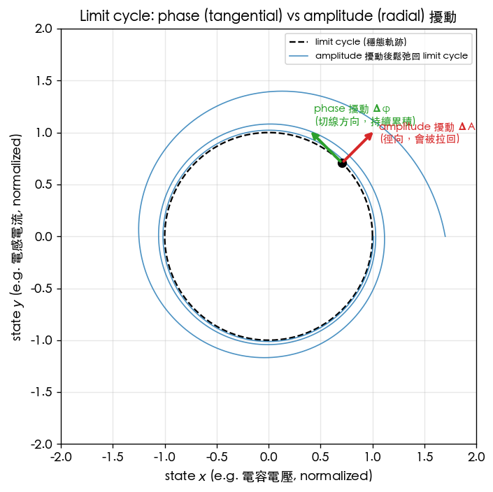
How to read this figure:

• Black dashed circle = the limit cycle (steady-state trajectory). The state point rotates counterclockwise along it at constant angular velocity $\omega_0$.
• Green arrow (tangential direction) = phase perturbation $\Delta\phi$: motion along the loop, equivalent to "arriving earlier or later at a given phase". No restoring force — it keeps accumulating.
• Red arrow (radial direction) = amplitude perturbation $\Delta A$: pushes the state point off (or into) the loop; the amplitude restoring term slowly pulls it back.
• The blue curve demonstrates the fate of a radial perturbation: starting from radius 1.7, it relaxes back to the unit circle within a few laps — the radial information is "forgotten".

Corresponding formula: project the perturbation vector $\delta\mathbf{z}$ onto the limit cycle's tangential unit vector $\hat{\mathbf{t}}$ (the phase direction) and radial unit vector $\hat{\mathbf{r}}$ (the amplitude direction) at that point:

$$\delta\mathbf{z}=\underbrace{(\delta\mathbf{z}\cdot\hat{\mathbf{t}})}_{\to\ \Delta\phi}\hat{\mathbf{t}}+\underbrace{(\delta\mathbf{z}\cdot\hat{\mathbf{r}})}_{\to\ \Delta A}\hat{\mathbf{r}}.$$

The tangential component determines the phase shift; the radial component determines the amplitude shift. The ISF is precisely the ratio function "how much of a unit injected charge ends up in the tangential component at a given injection phase" (formal definition in the impulse-to-phase-shift derivation).

Step 3: why an oscillator has no absolute time reference

This is the most crucial — and most often overlooked — sentence in the whole theory:

The differential equations of an autonomous oscillator contain no explicit time $t$.

That is, the equations only know "the state $\mathbf{z}$", not "what time it is". The mathematical consequence: if $\mathbf{z}(t)$ is a solution, then $\mathbf{z}(t-\Delta\tau)$, time-shifted by any constant $\Delta\tau$, is also a perfectly valid solution with the same energy and the same waveform.

• Math used: an autonomous system $\dot{\mathbf{z}}=F(\mathbf{z})$ is invariant under time translation (time-translation invariance). Displacement along the limit cycle corresponds exactly to this degree of freedom.
• Physical meaning: no external clock tells the oscillator "which phase it should be at". Sliding along the loop (= changing phase) costs no energy and is opposed by no restoring force. This is why phase is a marginally stable (neutrally stable) degree of freedom — corresponding to the system having one zero eigenvalue (Floquet exponent = 0).
• Contrast with amplitude: the direction perpendicular to the loop (amplitude) corresponds to a negative eigenvalue, so perturbations decay exponentially back onto the loop. (Rigorous Floquet/PPV theory is not among the 5 downloaded PDFs — it is external literature, e.g. Demir et al.; this site uses only the geometric intuition. See the supplementary note in effective_isf.)

One-sentence summary: phase is the only state direction of an oscillator with no restoring force, so noise affects phase permanently and cumulatively, whereas its effect on amplitude is temporary and gets absorbed.

Step 4: the same impulse, at a different injection phase, has a completely different effect

Since a perturbation decomposes into tangential and radial parts, where in the waveform you kick it determines the tangential/radial split. Take the pure sinusoid $V(t)=\cos(\omega_0 t)$:

• At the peak, $\theta=0$: the state point sits at the far right of the $x$ axis, and the state velocity (tangent) is purely along $y$. A voltage jump along $x$ is almost entirely radial — it changes only the amplitude, barely the phase. Corresponds to $\Gamma\approx 0$.
• At the zero crossing, $\theta=\pi/2$: the state point sits at the top of the $y$ axis, and the tangent is purely along $x$. The same voltage jump along $x$ is almost entirely tangential — it changes only the phase, barely the amplitude. Corresponds to maximum $|\Gamma|$.

The figure below draws this on the time-domain waveform:

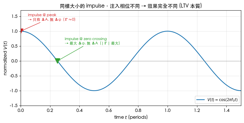
How to read this figure:

• The blue curve $V(t)=\cos(2\pi f_0 t)$ is the steady-state waveform.
• Red marker (peak): inject the impulse here → only $\Delta A$, almost no $\Delta\phi$ ($\Gamma\approx 0$).
• Green marker (zero crossing, where the slope is largest): inject the impulse here → maximum $\Delta\phi$, almost no $\Delta A$ (maximum $|\Gamma|$).
• Conclusion: phase sensitivity correlates strongly with "the waveform's instantaneous slope" — where the slope is large, the same voltage jump is equivalent to a larger time (phase) displacement. This is the geometric reason the ISF of an ideal LC comes out as $\Gamma(\theta)=-\sin\theta$ (a sinusoid has maximum slope at the zero crossings and zero slope at the peaks).

Corresponding formula (the operational ISF definition, [P1] Eq.(10)–(11), p.182; full derivation in the next chapter):

$$\Delta\phi=\frac{\Gamma(\omega_0\tau)}{q_{max}}\,\Delta q,\qquad \Gamma_{LC}(\theta)=-\sin\theta.$$

The fact "same impulse, different phase → different effect" goes by the formal name periodically time-varying sensitivity, and it is the core reason [P1] treats the oscillator as an LTV (linear time-variant) system (see LTI vs LTV).

Generating both figures with the real functions

Both figures are produced by simulations/lab_01_sinusoidal_oscillator.py. The limit cycle comes from the RK4 integration in simulate_lc() (with amplitude restoration); the waveform markers come from sinusoidal_oscillator():

from oscillator_models import simulate_lc, sinusoidal_oscillator
import numpy as np

# (1) limit cycle: start outside the loop (x0=1.7); the mu>0 amplitude restoring term pulls it back to the unit circle
t, x, y = simulate_lc(f0=1.0, t_end=3.0, fs=4000.0, mu=0.6, x0=1.7, y0=0.0)

# (2) pure sinusoid + peak / zero-crossing markers
tt = np.arange(int(2.0 * 4000.0)) / 4000.0
v  = sinusoidal_oscillator(tt, f0=1.0, amp=1.0)   # V = cos(2*pi*f0*t)
# peak  : theta=0      -> changes amplitude only (Gamma ~ 0)
# zero  : theta=pi/2 (t=0.25 T) -> changes phase only (|Gamma| max)

Full script: simulations/lab_01_sinusoidal_oscillator.py (core model: simulations/common/oscillator_models.py).

Parameter table:

Parameter	Symbol	Figure (limit cycle)	Figure (impulse markers)	Unit
Oscillation frequency	$f_0$	1.0 (normalized)	1.0 (normalized)	Hz
Sampling rate	$f_s$	4000	4000	Hz
Amplitude-restoring strength	$\mu$	0.6	— (pure sinusoid)	—
Initial state	$(x_0,y_0)$	$(1.7,\,0)$	—	normalized
Waveform amplitude	$A$	1 (steady-state radius)	1.0	normalized

Toy-model warning: both figures are pedagogical toy models — a normalized 2-D Van der Pol-style system reproducing the mechanism of "phase vs amplitude", not transistor-level real-circuit numbers. They correspond conceptually to [P1] Fig. 4 (impulse injected at peak vs zero crossing, the state-space limit cycle) and Sec. III-A, but the constants and waveforms are for teaching.

Step 5: amplitude error is pulled back, phase error accumulates → phase noise / jitter

Chaining the four steps together, look at the long-term consequence of noise kicking continuously:

1. Amplitude error: each time noise pushes the state slightly off the loop (radially), the amplitude restoring term pulls it back within a few time constants. Its effect on the output is bounded and decaying — which is why amplitude noise is usually suppressed naturally (see phase_vs_amplitude_noise).
2. Phase error: each time noise pushes the state slightly along the loop (tangentially), there is no restoring force, and that $\Delta\phi$ stays forever. The next noise kick adds another $\Delta\phi$… the phase performs a random walk.

Written in continuous form, this random walk is the next chapter's LTV convolution ([P1] Eq.(11), p.182):

$$\phi(t)=\frac{1}{q_{max}}\int_{-\infty}^{t}\Gamma(\omega_0\tau)\,i_n(\tau)\,d\tau.$$

The upper integration limit is $t$ (the system has memory), so the phase contributions of all past noise add up — this is the mathematical reason phase error accumulates, and the essence of phase noise/jitter.

The relation between phase noise and timing jitter

The same thing (the random wobble of phase) has two views, differing only by the conversion constant $2\pi f_0$:

• Phase noise: the frequency-domain view. Plot the power spectrum of the phase fluctuation: $S_\phi(f)$ (rad²/Hz), or the engineering-standard single-sideband (SSB) $\mathcal{L}(\Delta f)$ (dBc/Hz). The random walk of accumulated phase appears in the frequency domain as a $1/f^2$ skirt close to the carrier.
• Timing jitter: the time-domain view. Convert the phase error into "the timing error of an edge crossing zero", using $\Delta t=\Delta\phi/(2\pi f_0)$.

Conversion formulas (Eq.17 and Eq.19, Section 3 of the spec):

$$\Delta t=\frac{\Delta\phi}{2\pi f_0},\qquad \sigma_t=\frac{\sigma_\phi}{2\pi f_0}=\frac{1}{2\pi f_0}\sqrt{\int_{f_1}^{f_2}S_\phi(f)\,df}.$$

• Dimension check: $[\text{rad}]/[\text{rad/s}]=[\text{s}]$ ✓ (note that $2\pi f_0$ is in rad/s, not Hz).
• Random-walk signature: a phase random walk corresponds in the time domain to accumulated jitter $\sigma_{\Delta t}=\kappa\sqrt{\Delta t}$ ([P2] Eq.(8), p.792; κ from Eq.(12), p.793) — the longer the measurement interval, the larger the rms of the accumulated error, exactly the fingerprint of "no absolute time reference". See psd_phase_noise_jitter.

Numerical example (building intuition)

Using the canonical numbers of Section 8 of the spec, let us turn the geometry above into concrete figures.

Example A: $q_{max}=1$ pC, $\Delta q=1$ fC, $\Gamma=0.5$, $f_0=5$ GHz.

A charge impulse of $\Delta q=1$ fC injected at a phase where $\Gamma=0.5$ (between the peak and the zero crossing):

$$\Delta\phi=\frac{\Gamma\,\Delta q}{q_{max}}=\frac{0.5\times(1\times10^{-15}\,\text{C})}{1\times10^{-12}\,\text{C}}=5\times10^{-4}\ \text{rad}\;(\approx0.0286^\circ),$$

converted into a timing error:

$$\Delta t=\frac{\Delta\phi}{2\pi f_0}=\frac{5\times10^{-4}\ \text{rad}}{2\pi\times5\times10^{9}\ \text{Hz}}\approx1.59\times10^{-14}\ \text{s}=15.9\ \text{fs}.$$

• Feel for the numbers: at 5 GHz (period 200 ps), a 1 fC charge (about 6240 electrons) at a moderately sensitive phase causes only ~16 fs of timing error. Each kick is tiny, but phase has no restoring force, so as noise keeps kicking, the error integrates and accumulates — exactly the random walk of Step 5.
• If the same 1 fC lands on the peak ($\Gamma\approx 0$): $\Delta\phi\approx 0$, $\Delta t\approx 0$ — the energy goes almost entirely into amplitude and is absorbed by the restoring term within a few time constants, with no permanent effect on phase.

Applicability and failure conditions

Condition	When it holds	What happens when it fails
A stable limit cycle exists	Amplitude perturbations decay; only phase needs tracking	Without a stable loop (not yet oscillating, or multi-mode), the whole geometry does not apply
Small signal $\Delta q\ll q_{max}$	The tangential projection can be linearized, $\Delta\phi\propto\Delta q$	Large injection → nonlinearity, AM–PM, $\Gamma$ itself gets altered
Autonomous oscillation (no external clock)	Phase is a neutrally stable degree of freedom and accumulates	When phase-locked / injection-locked, phase is held by an external force (see [P3])
Impulse much narrower than the period $T$	It can be treated as an instantaneous voltage jump	Wide pulses require the integral form of Eq.(11)

Key takeaways

• The oscillator state, drawn in a 2-D plane, circles the limit cycle at constant speed; phase = the angular position along the loop.
• An autonomous oscillator has no absolute time reference (no explicit $t$ in the equations) → sliding along the loop costs no energy and is opposed by no restoring force.
• Perturbation decomposition: tangential = phase perturbation (accumulates permanently), radial = amplitude perturbation (pulled back by the restoring force).
• The same impulse at the peak ($\Gamma\approx 0$) vs at the zero crossing (maximum $|\Gamma|$) has drastically different effects → periodically time-varying sensitivity → the ISF.
• The accumulated phase random walk is, in the frequency domain, phase noise $\mathcal{L}(\Delta f)$; in the time domain, timing jitter $\sigma_t=\sigma_\phi/(2\pi f_0)$.
• Example A: 1 fC @ $\Gamma=0.5$, $q_{max}=1$ pC, 5 GHz → $\Delta\phi=5\times10^{-4}$ rad → 15.9 fs.
• Sources: [P1] Fig. 4, Sec. III-A; toy model from lab_01.

Further reading

• Next step — turning the geometry into formulas: From impulse to phase shift — the derivation
• Why phase noise matters and amplitude noise is suppressed: phase_vs_amplitude_noise
• The essence of periodically time-varying sensitivity: LTI vs LTV
• Site-wide symbols and units: Notation
• Numerical conversion practice: Numerical Feeling