β: This English translation is in beta — the Traditional-Chinese original is the authoritative version.

The DSP View of Phase Noise

Prerequisites: stochastic_noise_basics · white_noise_to_phase_noise ｜ Next: psd_phase_noise_jitter

The previous two pages computed phase noise from the circuit and from the frequency domain; this page puts on a different pair of glasses — re-examining the same thing from a signal-processing (DSP) viewpoint: treat the excess phase $\phi(t)$ as the output of a linear system whose input is the noise current, passing through two blocks: (1) a time-varying gain $\Gamma(\omega_0 t)/q_{max}$ (ISF weighting), and (2) an ideal integrator $\int dt$.

The payoff of this viewpoint is large: once you draw it as a block diagram, you immediately see that the $-20$ dB/dec (1/f²) slope of phase noise is no coincidence at all — it is simply the frequency response of the integrator. At the same time, this is the bridge that translates the continuous-time integral of [P1] Eq.(11) into the "discrete-time simulation code" (lab_06).

Physical intuition (big picture first): an integrator turns "something white" into "something that grows toward low frequency". Feed white noise through an integrator and the output PSD carries a $1/\omega^2$ — that is 1/f² phase noise. The ISF merely "phase-weights and downconverts" the input before the integration. Phase noise = ISF-weighted white noise, shaped by the integrator.

1. Reading [P1] Eq.(11) as a signal-processing chain

The central equation of [P1] (spec §3, formula 4):

$$\phi(t)=\frac{1}{q_{max}}\int_{-\infty}^{t}\Gamma(\omega_0\tau)\,i_n(\tau)\,d\tau .$$

The DSP decomposition: first define the "ISF-weighted equivalent noise current"

$$y(\tau)\equiv\frac{\Gamma(\omega_0\tau)}{q_{max}}\,i_n(\tau),$$

so that $\phi(t)=\int_{-\infty}^{t}y(\tau)\,d\tau$ — $\phi$ is the running integral of $y$. As a block diagram:

• Block B (ISF weighting) is LTV (linear time-varying): the gain varies periodically in time (period $T$) — this is the mathematical embodiment of [P1]'s emphasis that "an oscillator is time-variant, not time-invariant, toward noise" (claim C1). Its role is frequency translation: it "downconverts" noise near $n\omega_0$ to baseband ([P1] Eq.(13), Fig. 8).
• Block C (the integrator) is LTI (linear time-invariant): its frequency response is exactly $1/(j\omega)$.

2. Why the integrator 1/(jω) turns white noise into 1/f² (origin of the signature slope)

An ideal integrator $\phi(t)=\int y\,dt$ divides by $j\omega$ in the frequency domain:

$$\Phi(j\omega)=\frac{1}{j\omega}\,Y(j\omega)\quad\Longrightarrow\quad |H_{\text{int}}(j\omega)|^2=\frac{1}{\omega^2}.$$

The rule for PSDs through a linear system is $S_{\text{out}}=|H|^2\,S_{\text{in}}$. If the ISF-weighted equivalent input $y$ is approximately white in the offset band we care about (power $\propto\Gamma_{rms}^2 S_i/q_{max}^2$), then:

$$\boxed{\ S_\phi(\Delta\omega)=|H_{\text{int}}|^2\,S_y=\frac{1}{\Delta\omega^2}\cdot\frac{\Gamma_{rms}^2}{q_{max}^2}\,S_i\ }$$

• dimension check: $[1/(\text{rad/s})^2]\times[(\text{rad}^2)\cdot\text{A}^2/\text{Hz}/\text{C}^2]$. $\Gamma$ is dimensionless, $q_{max}$ is C, $S_i$ is $\text{A}^2/\text{Hz}=\text{C}^2/(\text{s}^2\cdot\text{Hz})$; collecting terms gives $\text{rad}^2/\text{Hz}$ (treating the rad² in $1/(\text{rad/s})^2$ as phase rad²), consistent with the units of $S_\phi$ ✓.
• This is the 1/f²: $S_\phi\propto1/\Delta\omega^2$, i.e. $-20$ dB/dec on a log-log plot. Expressed in dBc/Hz ($\mathcal{L}\approx\frac12 S_\phi$), the skirt is still $-20$ dB/dec.
• Comparison with [P1] Eq.(21) (including the famous factor-of-2): the clean time-domain derivation "white noise × ISF → integrate" gives $\mathcal{L}=\Gamma_{rms}^2 S_i/(2q_{max}^2\Delta\omega^2)$, whereas [P1] Eq.(21) is written with $/(4\Delta\omega^2)$. The factor of 2 comes purely from the SSB bookkeeping convention ($\mathcal{L}\approx\frac12 S_\phi$), and does not affect the $\Gamma_{rms}^2/q_{max}^2$ scaling or the $-20$ dB/dec slope. Full discussion in white_noise_to_phase_noise.
• Extension to flicker: if the input is not white but 1/f ([P1] Eq.(22)), the same $1/\omega^2$ integrator produces $1/\omega^3$ at the output — the close-in 1/f³ phase noise ([P1] Eq.(23)). The DSP view unifies "1/f² and 1/f³" as "the same integrator acting on inputs of different colors".

This also explains "why phase accumulates but amplitude does not": the integrator has infinite DC gain ($1/\omega\to\infty$ when $\omega\to0$), so phase is infinitely sensitive to very-low-frequency perturbations and random-walks away (no restoring force); the amplitude path instead has a decaying (restoring) pole — high-pass / finite gain — so perturbations get pulled back. Compare phase_vs_amplitude_noise (claim C2).

3. From continuous time to discrete simulation: turning the formula into code (lab_06)

To verify the theory on a computer, the continuous integral must be replaced by a discrete accumulation. With sampling frequency $f_s$ and interval $\Delta t_s=1/f_s$, the discrete version of [P1] Eq.(11) is a cumulative sum:

$$\phi[k]=\frac{\Delta t_s}{q_{max}}\sum_{m=0}^{k}\Gamma(\omega_0\,m\,\Delta t_s)\,i_n[m].$$

• The role of $\Delta t_s$: it calibrates the "discrete sum" back to the physical dimensions of an "integral". Dropping $\Delta t_s$ is the most common discretization mistake (the units end up off by a factor of $f_s$).
• PSD of discrete white noise: to generate a white sequence with single-sided PSD $S_i$, the variance of each sample must be set to $\sigma^2=S_i\cdot f_s/2$ (the single-to-double-sided factor of 2 and the sampling bandwidth $f_s/2$). This constant must match the analytic expression, or the numerics will not lie on the theory line.
• cumsum = the integrator: numpy.cumsum is the discrete integrator; its frequency response approaches $1/\omega$ at low frequency — exactly the source of our 1/f².

The corresponding core code (using the real functions of spec §5):

import numpy as np
from simulations.common.noise_utils import white_noise, estimate_psd
from simulations.common.isf_utils import apply_isf_weighting, gamma_lc_ideal

# 0) time axis
t = np.arange(N) / fs

# 1) generate the white noise-current sequence i_n[m], single-sided PSD = S_i
i_n = white_noise(n=N, psd=1e-24, fs=fs, rng=rng)          # A, white

# 2a) ISF weighting (time-varying multiply only, with NO integration): y[m] = Gamma(w0 t)/qmax * i_n
y = apply_isf_weighting(t, i_n, gamma_func=gamma_lc_ideal, qmax=1e-12, omega0=2*np.pi*5e9)

# 2b) integrator: phi[k] = dt * cumsum(y) — cumsum×dt is the true discrete integral
dt = 1.0 / fs
phi = np.cumsum(y) * dt

# 3) Welch PSD estimate, verify S_phi ∝ 1/f^2
f, S_phi = estimate_psd(phi, fs=fs, nperseg=4096)

Full script: simulations/lab_06_white_noise_phase_noise.py (see lab_06). This is a pedagogical toy model (ideal-LC $\Gamma=-\sin\theta$, a single white-noise source), not transistor-level.

4. Welch PSD estimation: how to "measure" S_φ(f)

You have simulated a time series $\phi[k]$; how do you recover its PSD $S_\phi(f)$ to compare against the theoretical 1/f²? A single FFT with the squared magnitude (the periodogram) has an estimator variance that does not decrease as the record gets longer — the estimate stays wildly noisy. Welch's method solves this:

1. Split the long sequence into segments (each nperseg points long), optionally overlapping (typically 50%).
2. Multiply each segment by a window (a window function, e.g. Hann, to suppress spectral leakage).
3. Take the periodogram of each segment, then average. Averaging $K$ segments lowers the estimator variance by about $1/K$.

• trade-off: shorter segments → more segments to average, smoother, but worse frequency resolution ($\Delta f\approx f_s/\text{nperseg}$) — the close-in 1/f² details get smeared out. Longer segments → better resolution but noisier. Seeing the close-in 1/f² requires long segments + long records.
• This site uses estimate_psd(x, fs, nperseg) (spec §5, noise_utils) for this; the lab_06 figure overlays the Welch estimate (dots) on the analytic 1/f² line (solid), and the two agree.

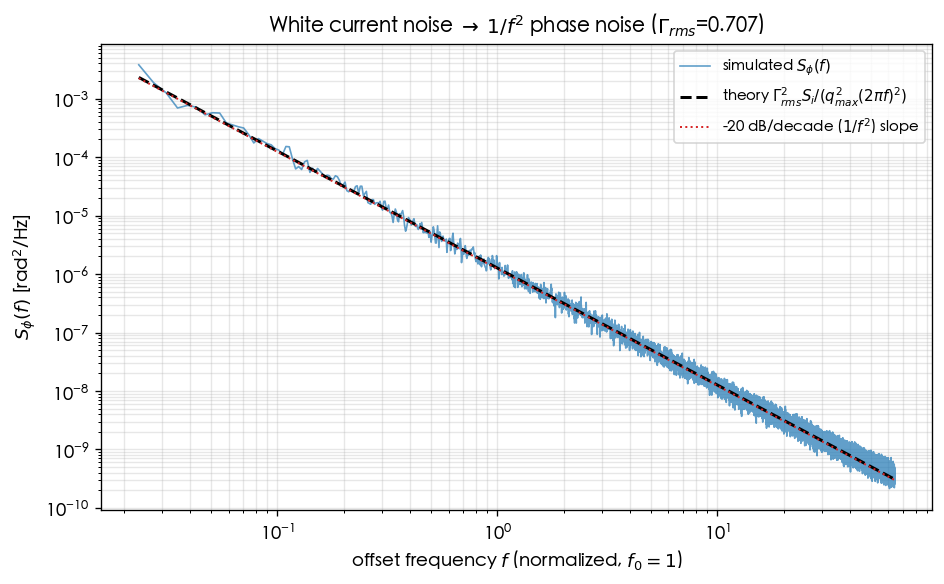
The figure above (simulations/lab_06_white_noise_phase_noise.py, corresponding to spec §4 white_noise_phase_noise_psd.png) is the "seeing is believing" of this DSP chain: white-noise input → ISF weighting → cumsum integrator → Welch estimate, giving an $S_\phi$ that is a clean $-20$ dB/dec on log-log, coinciding with the analytic $1/\Delta\omega^2$ of Section 2.

5. Sampling and aliasing: the easiest traps to step into from the DSP viewpoint

When moving a continuous system into a discrete simulation, aliasing (frequencies above Nyquist folding back to low frequency and masquerading as others) is the number-one pitfall, and ISF simulations require particular care:

• The Nyquist iron law: $f_s$ must be $\ge2\times$ the highest signal frequency. The ISF weighting contains $\Gamma(\omega_0 t)$ and its harmonics $n\omega_0$, so your $f_s$ must be not merely $>2f_0$ but ideally $\gg f_0$ (covering the few ISF harmonics $n\omega_0$ you care about); otherwise the downconversion of higher harmonics gets contaminated by aliasing, and the 1/f² line kicks up at high offsets.
• White noise is inherently aliased: ideal white noise has infinite bandwidth, and discrete sampling inevitably folds all frequencies into $[0,f_s/2]$. That is fine — as long as $f_s$ is high enough and we only interpret the offset band $\ll f_s/2$. When reporting a PSD, trust only the band far below Nyquist.
• The integrator's DC singularity: $1/\omega$ diverges as $\omega\to0$; a discrete cumsum manifests as a random walk (unbounded drift). In simulation, either look only at a finite offset band or detrend $\phi$; otherwise the lowest few PSD bins are dominated by drift — this is exactly the numerical version of "$\phi$ is not stationary; do statistics on phase differences/frequency" mentioned in Section 5 of stochastic_noise_basics.

6. Continuous ↔ discrete correspondence table

Continuous time ([P1])	Discrete simulation (lab_06)	Caveats
$\int_{-\infty}^{t}(\cdot)\,d\tau$	numpy.cumsum(...) * dt	do not drop $\Delta t_s=1/f_s$
$\Gamma(\omega_0\tau)$ time-varying gain	gamma_func(omega0 * t) pointwise multiply	LTV: a different gain per sample
white PSD $S_i$ ($\text{A}^2/\text{Hz}$)	sample variance $\sigma^2=S_i f_s/2$	single↔double-sided factor of 2
$1/(j\omega)$ integrator → 1/f²	low-frequency response of cumsum	DC singularity → drift; detrend
theoretical $S_\phi(f)$ curve	estimate_psd (Welch)	segment length vs resolution trade-off
continuous frequency $\Delta\omega$	bin frequency $f<f_s/2$	trust only bands far below Nyquist

Applicability and failure conditions

Condition	When it holds	When it fails
Linear superposition (small perturbations)	$S_{\text{out}}=\lvert H\rvert^2 S_{\text{in}}$ applies	large injection is nonlinear, AM–PM; must remodel
$f_s\gg f_0$ and covers the harmonics of interest	clean 1/f² line	aliasing folds high harmonics back; high offsets kick up
Interpret only offsets $\ll f_s/2$	PSD trustworthy	bins near Nyquist untrustworthy
Welch segment length matched to the band of interest	close-in 1/f² resolved	segments too short smear low offsets; too long, too noisy
Detrend $\phi$ / use phase differences	avoids the random-walk drift	FFT of raw $\phi$: lowest bins dominated by drift

Corresponding papers / formulas

• The phase integral (decomposed by DSP into "ISF weighting + integrator"): [P1] Eq.(11), p.182 (spec formula 4).
• LTV / frequency translation (ISF harmonic downconversion): [P1] Eq.(13), Fig. 8, p.183 (claim C1).
• The signature white noise → 1/f² result: [P1] Eq.(21), p.185; factor-of-2 note in spec §3.
• flicker → 1/f³ (the same integrator acting on a 1/f input): [P1] Eqs.(22),(23), p.185.
• Figure: white_noise_phase_noise_psd.png (lab_06), corresponding to spec §4.
• The DSP tools (Welch / aliasing / windowing) are standard signal processing, not among the 5 source PDFs; supplied from standard references.

Key takeaways

• The DSP model of phase noise: white noise $\to$ ISF time-varying weighting (LTV, frequency translation) $\to$ integrator $1/(j\omega)$ (LTI) $\to\phi$.
• The integrator's $|H|^2=1/\omega^2$ is the source of the 1/f² ($-20$ dB/dec) slope; a 1/f input → 1/f³.
• Discretization: integral = cumsum × dt; white-noise variance $=S_i f_s/2$; do not drop $\Delta t_s$.
• Welch PSD: segment + window + average to lower the estimator variance; trade segment length against resolution.
• Aliasing: $f_s\gg f_0$ and cover the harmonics of interest; trust only offsets $\ll f_s/2$; detrend $\phi$ to avoid drift domination.
• Matches the analytic result (lab_06 figure); the factor of 2 is just SSB bookkeeping and changes neither the scaling nor the slope.

Further reading

• The analytic white noise → 1/f² (with the factor-of-2 discussion): white_noise_to_phase_noise
• Stochastic-process prerequisites (PSD / Parseval / cyclostationary): stochastic_noise_basics
• Converting phase noise into jitter: psd_phase_noise_jitter
• Simulation lab: lab_06
• Why phase integrates while amplitude decays: phase_vs_amplitude_noise