Why phase noise matters and why amplitude noise is suppressed

β: This English translation is in beta — the Traditional-Chinese original is the authoritative version.

Prerequisites: oscillator_phase · Unified notation table | Next: lti_vs_ltv

The previous page, oscillator_phase, showed geometrically that a noise perturbation to an oscillator decomposes into a tangential (phase) component and a radial (amplitude) component. This page answers the two most practical engineering questions:

1. Why do we worry almost exclusively about phase noise, and hardly at all about amplitude noise?
2. Can the fact that "amplitude perturbations get pulled back" be written as a sensitivity function, just like the ISF?

The key term in the answer is the APF (Amplitude Perturbation Function) — introduced by [P4] as the amplitude-domain counterpart of the ISF.

Physical intuition (conclusion first): the limit cycle's "stability" is completely different in the two directions. The radial (amplitude) direction has a restoring force (negative Floquet exponent): perturbations decay exponentially back onto the cycle, so the oscillator suppresses amplitude noise by itself. The tangential (phase) direction has no restoring force (zero Floquet exponent): perturbations accumulate permanently, so phase noise random-walks without bound. For one and the same noise current, the share injected into phase stays, and the share injected into amplitude gets eaten — the ISF $\Gamma$ describes "how much goes into phase", the APF $\Lambda$ describes "how much goes into amplitude".

1. Why phase noise matters

Write the oscillator output in the standard decomposition ([P1] Eq.(1), p.181):

$$V_{out}(t)=A(t)\,f\!\big(\omega_0 t+\phi(t)\big).$$

Here $A(t)$ is the instantaneous amplitude, $\phi(t)$ is the excess phase (the deviation beyond the ideal phase), and $f$ is the periodic steady-state waveform. The noise hides inside the two modulations $A(t)$ and $\phi(t)$. Their impact on "clock quality" is asymmetric:

• Phase noise turns directly into timing jitter: clocked circuits care about "when the edge crosses the threshold". That instant is set by phase: $\Delta t=\Delta\phi/(2\pi f_0)$. Phase jitter = edge timing jitter = SerDes eye closure and mis-timed sampling.
• Phase errors accumulate, with no upper bound: since phase has no restoring force (Step 3 of the previous page), $\phi(t)$ performs a random walk and its variance grows with time. In the frequency domain this shows up as the tall $1/f^2$ (and, closer in, $1/f^3$) skirts beside the carrier. This is the fundamental reason the oscillator spectrum is not an ideal delta but has finite width.
• Amplitude errors are bounded, and mostly never reach the threshold decision: near the threshold, amplitude effects mostly convert back into timing error (see AM–PM below), but pure amplitude fluctuations themselves are squeezed out by the restoring force, and receivers commonly use limiters/comparators that are insensitive to amplitude.

In one sentence: for communication and clocking systems, timing jitter = a phase matter. That is why the entire Hajimiri–Lee theory bets everything on $\phi(t)$ and first "legitimately throws away" the amplitude degree of freedom — the next section explains why that is allowed.

2. Why amplitude perturbations decay: the APF and the amplitude decay function

The ISF writes "injected charge → phase shift" as ([P1] Eq.(10), p.182)

$$\Delta\phi=\frac{\Gamma(\omega_0\tau)}{q_{max}}\,\Delta q.$$

[P4] does the exact parallel for amplitude, defining the APF $\Lambda(\phi)$ (amplitude perturbation function): the same injected current impulse, projected onto the radial direction of the limit cycle, produces how much instantaneous amplitude deviation. Conceptually ([P4] Sec. III-D; the APF is defined near p.2127):

$$\Delta A_0\;\propto\;\Lambda(\omega_0\tau)\,\Delta q \quad\Longleftrightarrow\quad \text{the APF is the amplitude-domain counterpart of the ISF}.$$

• Units: [P4] gives the APF units of $\mathrm{A^{-1}}$ (1/ampere) — it maps "injected current" to "relative amplitude deviation". Contrast the dimensionless ISF $\Gamma$: the two are structurally parallel but normalized differently.
• The key difference — different fates: the phase deviation carries a unit step $u(t-\tau)$ (kept forever, [P1] Eq.(10)); the amplitude deviation is instead multiplied by an amplitude decay function that relaxes exponentially back to zero. Conceptually:

$$\underbrace{h_\phi(t,\tau)=\frac{\Gamma(\omega_0\tau)}{q_{max}}\,u(t-\tau)}_{\text{phase: step, permanent}}\qquad\text{vs}\qquad \underbrace{h_A(t,\tau)\;\propto\;\Lambda(\omega_0\tau)\,d(t-\tau)}_{\text{amplitude: impulse}\times\text{decay,}\;d\to 0}.$$

Here $d(t-\tau)$ is the amplitude decay function. [P4] Sec. III-F, p.2128 (the body text immediately before Eq.(25)) gives the exact closed form (verified verbatim against the original PDF rendering; note that Eq.(25) itself is $\Lambda(\phi)=\tau_0\,\tilde\Lambda(\phi)$, APF = $\tau_0$ × amplitude ISF, while the decay closed form below is the body text preceding it):

$$d(t,\phi)=e^{-t/\tau_0},\qquad \tau_0=\frac{2Q}{\omega_{osc}}$$

That is, $\tau_A=\tau_0=2Q/\omega_{osc}$ — the amplitude recovery time constant is proportional to $Q$. Intuition: a high-$Q$ LC recovers its amplitude slowly ($\tau_0$ large), but it does eventually recover (exponential decay); phase has no such restoring force (unit step, infinitely long memory). This is the most quantitative one-liner for "why amplitude noise is bounded while phase noise diverges".

Verified: $d(t,\phi)=e^{-t/\tau_0}$ and $\tau_0=2Q/\omega_{osc}$ come from the body text of [P4] Sec. III-F, p.2128 (the unnumbered expression immediately before Eq.(25); Eq.(25) itself is the APF relation $\Lambda(\phi)=\tau_0\,\tilde\Lambda(\phi)$). (Decay rates for more general oscillators belong to the Floquet/PPV framework, not among the 5 downloaded PDFs; see derivation_floquet_ppv.)

• Why "decays" equals "suppressed": think of amplitude noise as a convolution with $h_A$. Because $d(t-\tau)$ is integrable and returns to zero, past amplitude perturbations do not accumulate, and the output amplitude variance converges to a finite value (the steady-state variance of a first-order low-pass system with a restoring force). Phase convolution instead uses $u(t-\tau)$ (non-integrable, never returns to zero), so the variance diverges — this is the mathematical watershed between phase noise accumulating and amplitude noise not accumulating.

Putting the ISF and the APF side by side, condensing the whole page cell by cell:

Quantity	Projection direction	Sensitivity function	Impulse-response kernel	Long-term fate	Effect on jitter
Phase $\phi$	Tangential (along the cycle)	ISF $\Gamma(\omega_0\tau)$, dimensionless	$\dfrac{\Gamma}{q_{max}}u(t-\tau)$ (step)	Accumulates / diverges	Direct: $\Delta t=\Delta\phi/2\pi f_0$
Amplitude $A$	Radial (perpendicular to the cycle)	APF $\Lambda(\omega_0\tau)$, units $\mathrm{A^{-1}}$	$\Lambda\cdot d(t-\tau)$ (impulse × decay)	Decays / bounded	Indirect, mostly via AM–PM

3. Ideal LC: ISF and APF in quadrature (90° apart)

[P4] Fig. 5, p.2126 plots, for the ideal LC oscillator, the ISF, APF, amplitude decay function, and how the three relate; the most elegant conclusion is:

In the ideal LC oscillator, the ISF and the APF are in quadrature (90° apart).

This matches the geometry of the previous page exactly: tangential and radial are everywhere mutually perpendicular on the circle. The ideal LC's ISF is $\Gamma(\theta)=-\sin\theta$ (maximal at the zero crossings, zero at the peaks); the radial sensitivity (APF) should then be maximal at the peaks and zero at the zero crossings, i.e. shaped like $\cos$:

$$\Gamma_{LC}(\theta)=-\sin\theta\quad\text{(tangential)},\qquad \Lambda_{LC}(\theta)\;\propto\;\cos\theta\quad\text{(radial, orthogonal to }\Gamma\text{)}.$$

• Physical meaning: kick at the peak ($\theta=0$) → $\Gamma=0$, $\Lambda$ maximal → pure amplitude change (gets eaten). Kick at the zero crossing ($\theta=\pi/2$) → $|\Gamma|$ maximal, $\Lambda=0$ → pure phase change (kept forever). This is exactly the red/green markers in the previous page's waveform_with_impulse_markers.
• Unit check / dimension: $\Gamma$ is dimensionless, $\Lambda$ has units $\mathrm{A^{-1}}$; quadrature refers to the phase (angle) relation, not equal dimensions. "90° apart" means that, as periodic functions of $\theta$, one is a $\sin$ and the other a $\cos$ in Fourier terms.

Verified ([P4] Eq.(26), p.2128): the proportionality constant in $\Lambda_{LC}\propto\cos\theta$ above and the exact normalization of the APF must be checked against PDF Fig. 5, p.2126. This page only claims the qualitative quadrature relation (stated explicitly by [P4]) and does not pin down the amplitude constant.

4. AM–PM in brief: the back door through which amplitude noise leaks into phase

If amplitude perturbations get eaten, why should design still care about them? Because there is a back door called AM–PM conversion (amplitude-to-phase conversion):

• Mechanism: a real oscillator's effective oscillation frequency varies with amplitude (e.g. a nonlinear capacitance $C(V)$ that changes with swing, or a tank whose effective phase shifts with amplitude). So "amplitude fluctuation $\Delta A$" leaks through $\dfrac{\partial\omega}{\partial A}$ into "phase/frequency fluctuation", which the phase's lack of restoring force then accumulates permanently.

• Consequence: amplitude noise that should have been squeezed out becomes long-lived phase noise via AM–PM — in particular, it upconverts the device's $1/f$ amplitude fluctuations into close-in phase noise, degrading the $1/f^3$ region.

• Design implications: (i) drive $\partial\omega/\partial A\to 0$ (e.g. bias at a flat spot of the capacitance curve, add AM suppression/limiting); (ii) under the quadrature picture, arranging the dominant noise injection at the phases where the radial direction is least sensitive also helps. The detailed AM–PM and amplitude-modulation analysis is the core of [P4] (advanced — this site gives only the intuition).

• Connections to other pages on this site: AM–PM is one of the common reasons "why the real $1/f^3$ sits higher than the pure $c_0$ mechanism predicts"; for the purely ISF-$c_0$ upconversion of $1/f$, see flicker_upconversion and [P1] Eq.(23)–(24).

Numerical example (building intuition)

Adapted from Example A: $q_{max}=1$ pC, $\Delta q=1$ fC, $f_0=5$ GHz; compare the long-term consequences of injecting at the zero crossing ($\Gamma=-1$, pure phase) versus at the peak ($\Gamma\approx 0$, pure amplitude).

Injection at the zero crossing ($\theta=\pi/2$, $\Gamma=-\sin(\pi/2)=-1$):

$$\Delta\phi=\frac{|\Gamma|\,\Delta q}{q_{max}}=\frac{1\times10^{-15}}{10^{-12}}=1\times10^{-3}\ \text{rad}\ \Rightarrow\ \Delta t=\frac{10^{-3}}{2\pi\times5\times10^{9}}\approx31.8\ \text{fs (kept permanently)}.$$

Injection at the peak ($\theta=0$, $\Gamma\approx 0$): $\Delta\phi\approx 0$; nearly all the energy goes into amplitude. The amplitude deviation $\Delta A$ relaxes back to zero after a few $\tau_A$ (the amplitude recovery time constant), with no permanent effect on phase (unless the AM–PM back door is open).

• Dimension check: $[\text{rad}]/[\text{rad/s}]=[\text{s}]$ ✓.
• Feel for the numbers: for the same 1 fC, a 90° difference in injection phase is the difference between "31.8 fs of permanent jitter" and "~0 permanent effect". This makes very concrete "why the shape of the phase sensitivity (ISF) matters so much" — placing the noise sources at the phases where the phase is least sensitive ($\Gamma$ small) lowers phase noise for free.

Validity and failure conditions

Condition	When it holds	When it fails
Amplitude restoration present (stable limit cycle)	Amplitude noise decays; tracking phase alone suffices	With weak restoration / slow high-Q recovery, amplitude noise lives longer and cannot be ignored
AM–PM negligible ($\partial\omega/\partial A\approx 0$)	"Discard amplitude" is a good approximation	With strong AM–PM, amplitude noise upconverts into phase noise; use the [P4] APF framework
Small-signal perturbation	$\Gamma,\Lambda$ project linearly	Large injection alters the ISF/APF themselves; nonlinear mixing
Ideal LC symmetry	$\Gamma\perp\Lambda$ (quadrature) holds	For asymmetric waveforms / rings, quadrature is only approximate

5. The amplitude-noise spectrum: OU process and the flat-top Lorentzian

Section 2 described the fate of a single kick: the amplitude deviation decays as $d(t)=e^{-t/\tau_0}$ with $\tau_0=2Q/\omega_{osc}$ ([P4] Sec. III-F, p.2128, verified on this site). But real noise is not a single kick — it is a continuous stream of white-noise current. This section upgrades "single-kick decay" to "the steady-state spectrum under continuous drive", answering two questions:

1. What does the full amplitude-noise spectrum $S_a(\omega)$ look like? (Answer: a "flat-top Lorentzian" with the corner at $\omega_0/2Q$.)
2. Why does the measured oscillator spectrum "flatten" far from the carrier? Besides the instrument floor there is a second physical reason — the AM plateau.

Physical intuition (conclusion first): white noise = a dense stream of small random kicks. On the phase side every kick is kept forever (unit step) → they pile up into a random walk → spectrum $\propto 1/\omega^2$ all the way down. On the amplitude side every kick carries an $e^{-t/\tau_0}$ "shelf life" → after superposition only the kicks within the last $\tau_0$ are still alive → finite variance, spectrum flattens for $\omega \lt 1/\tau_0$. At observation frequencies above $1/\tau_0$ (time scales shorter than $\tau_0$) the restoring force has no time to act and the amplitude also looks like a free integrator — so at the high-frequency end the AM and PM spectra have the same shape.

5.1 From a single kick to continuous drive: the Langevin / OU equation

Linearize the amplitude dynamics of Section 2 (small perturbation): the restoring force pulls the amplitude deviation back at rate $1/\tau_0$ while white noise keeps pushing it. Define $a(t)\equiv \Delta A/A_0$ as the relative amplitude deviation (dimensionless, so it can be compared fairly with $\phi$ [rad]); its stochastic differential equation (Langevin equation) is:

$$da=-\frac{a}{\tau_0}\,dt+\sqrt{c}\,dW(t).$$

Term by term, physical meaning and units:

• $-\dfrac{a}{\tau_0}dt$: the restoring term — the linearization of amplitude control (limiting, nonlinear saturation), precisely the differential form of [P4]'s single-kick decay $d(t)=e^{-t/\tau_0}$. $[a/\tau_0]\cdot[dt]=(1/\text{s})\cdot\text{s}$ × dimensionless = dimensionless ✓. $\tau_0=2Q/\omega_0$ [s] ([P4] Sec. III-F, p.2128, verified).
• $\sqrt{c}\,dW$: the white-noise drive. $W(t)$ is a standard Wiener process, $\mathrm{Var}[dW]=dt$, $[dW]=\sqrt{\text{s}}$; $c$ is the drive strength, $[c]=1/\text{s}$ (with $a$ dimensionless), so $[\sqrt{c}\,dW]=\sqrt{1/\text{s}}\cdot\sqrt{\text{s}}=$ dimensionless ✓.
• The phase equation = the same equation with the restoring term removed: $d\phi=\sqrt{c}\,dW$ ($[c]=\text{rad}^2/\text{s}$). This is the minimal mathematical model of "one white-noise source, two fates".

A process of this kind — "exponential restoration + white-noise drive" — is called an Ornstein–Uhlenbeck (OU) process.

Honesty note: the OU process and the solution below are standard stochastic-process mathematics (external literature, not among the 5 source PDFs): G. E. Uhlenbeck and L. S. Ornstein, "On the Theory of the Brownian Motion," Physical Review, vol. 36, pp. 823–841, 1930. The only ingredient taken from the papers on this site is the decay time constant $\tau_0=2Q/\omega_0$ ([P4] Sec. III-F, p.2128, verified verbatim); plugging it into the OU machinery is a standard pedagogical assembly.

5.2 Solving the OU process: autocorrelation and finite variance (step by step)

Step 1: solve the SDE with an integrating factor. Differentiate $e^{t/\tau_0}a$:

$$d\!\left(e^{t/\tau_0}a\right)=e^{t/\tau_0}\left(da+\frac{a}{\tau_0}dt\right)=e^{t/\tau_0}\sqrt{c}\,dW,$$

integrate both sides from $-\infty$ to $t$ (steady state: the initial condition has long since decayed away):

$$a(t)=\sqrt{c}\int_{-\infty}^{t}e^{-(t-s)/\tau_0}\,dW(s).$$

Physical meaning: the present amplitude deviation = every past kick ($dW(s)$), each weighted by its own decay $e^{-(t-s)/\tau_0}$, superposed — exactly the result of convolving Section 2's [P4] $d(t)$ with the noise, in sharp contrast with the phase side $\phi(t)=\sqrt{c}\int^t dW$ (every kick keeps weight 1 forever).

Step 2: autocorrelation. Using "$dW$ at different times are uncorrelated, $\mathrm{E}[dW^2]=ds$" (the Itô isometry, a standard result), for $\tau\ge 0$:

$$\begin{aligned} R_a(\tau)&\equiv \mathrm{E}[a(t)\,a(t+\tau)] =c\int_{-\infty}^{t}e^{-(t-s)/\tau_0}\,e^{-(t+\tau-s)/\tau_0}\,ds\\ &=c\,e^{-\tau/\tau_0}\int_{-\infty}^{t}e^{-2(t-s)/\tau_0}\,ds =c\,e^{-\tau/\tau_0}\cdot\frac{\tau_0}{2} \qquad(\text{substitute }u=t-s,\ \int_0^\infty e^{-2u/\tau_0}du=\tfrac{\tau_0}{2}), \end{aligned}$$ $$\boxed{\ R_a(\tau)=\frac{c\,\tau_0}{2}\,e^{-\lvert\tau\rvert/\tau_0}\ }$$

Step 3: the variance is finite. $\mathrm{Var}[a]=R_a(0)=c\tau_0/2$. Units: $(1/\text{s})\cdot\text{s}=$ dimensionless ✓ ($a^2$). Compare phase: $\mathrm{Var}[\phi(t)]=c\,t$ diverges linearly in time (random walk; see the $2D\lvert t\rvert$ of lorentzian_linewidth, corresponding to $c=2D$). "Finite vs divergent" variance is the steady-state version of Section 2's "decaying kernel vs step kernel".

5.3 Wiener–Khinchin → flat-top Lorentzian (step-by-step integration)

The PSD of a stationary process is the Fourier transform of its autocorrelation (Wiener–Khinchin, a standard result). First compute the transform of $e^{-\lvert\tau\rvert/\tau_0}$ (same trick as on the Lorentzian linewidth page — split the absolute value into two halves):

$$\int_{-\infty}^{\infty}e^{-\lvert\tau\rvert/\tau_0}e^{-j\omega\tau}\,d\tau =\frac{1}{1/\tau_0+j\omega}+\frac{1}{1/\tau_0-j\omega} =\frac{2/\tau_0}{1/\tau_0^2+\omega^2} =\frac{2\tau_0}{1+\omega^2\tau_0^2}.$$

Multiply by the prefactor $c\tau_0/2$ of $R_a$:

$$\boxed{\ S_a(\omega)=\frac{c\,\tau_0^2}{1+\omega^2\tau_0^2}\ }\qquad\left[\frac{1}{\text{Hz}}\right]$$

• Convention (factor-of-2 discipline): this section uses the two-sided PSD throughout ($\pm\infty$ integrals, inverse transform carrying $1/2\pi$). The scipy.signal.welch used in the simulation returns the one-sided PSD = 2× two-sided, so the theory lines on the lab_28 plots are $2c/\omega^2$ and $2c\tau_0^2/(1+\omega^2\tau_0^2)$. Corner frequencies, crossover frequencies, and PM/AM ratios are all obtained as ratios, hence completely insensitive to one-sided/two-sided or to the $\mathcal{L}=S_\phi/2$ vs /4 convention — only absolute dBc/Hz values require stating the convention (see 5.6).
• Unit check: $[c\tau_0^2]=(1/\text{s})\cdot\text{s}^2=\text{s}=1/\text{Hz}$ ✓ (PSD of a dimensionless quantity).
• Two limits (shape):
  • $\omega\tau_0\ll 1$ (low frequency): $S_a\to c\tau_0^2$, flat top. The restoring force has time to lock the variance down.
  • $\omega\tau_0\gg 1$ (high frequency): $S_a\to c/\omega^2$, identical to a free integrator. On time scales shorter than $\tau_0$ the restoring force simply has no time to act.
• Corner: the two asymptotes intersect at $$\omega_c=\frac{1}{\tau_0}=\frac{\omega_0}{2Q}\ \ [\text{rad/s}] \qquad\Longleftrightarrow\qquad f_c=\frac{\omega_c}{2\pi}=\frac{f_0}{2Q}\ \ [\text{Hz}],$$ and at the corner $S_a=c\tau_0^2/2$ (3 dB below the flat top). In Hz, remember $f_c=f_0/2Q$.
• Power-conservation self-check: $\dfrac{1}{2\pi}\displaystyle\int_{-\infty}^{\infty} \frac{c\tau_0^2\,d\omega}{1+\omega^2\tau_0^2}=\frac{c\tau_0^2}{2\pi}\cdot\frac{\pi}{\tau_0} =\frac{c\tau_0}{2}=\mathrm{Var}[a]$ ✓ (integral formula $\int d\omega/(1+\omega^2\tau_0^2)=\pi/\tau_0$).

This shape is called a flat-top Lorentzian: it belongs to the same family of functions as the carrier lineshape $D/(D^2+\Delta\omega^2)$ of the lorentzian_linewidth page, but the physical protagonist differs — there it is "the carrier lineshape caused by the phase random walk" (corner $=D$, very narrow); here it is "the AM-noise spectrum caused by the amplitude restoring force" (corner $=\omega_0/2Q$, very wide).

5.4 Contrast with phase: no restoring force, $1/\omega^2$ all the way down

The same white-noise source driving phase: $d\phi=\sqrt{c}\,dW$, i.e. $\phi$ is the integral of white noise. The integrator $\lvert H(j\omega)\rvert^2=1/\omega^2$ acting on white noise of two-sided level $c$:

$$S_\phi(\omega)=\frac{c}{\omega^2}\qquad\left[\frac{\text{rad}^2}{\text{Hz}}\right].$$

Cell-by-cell comparison ($\lvert\cdot\rvert$ in the table denotes absolute value):

	Phase $\phi$	Amplitude $a$
Equation	$d\phi=\sqrt{c}\,dW$	$da=-(a/\tau_0)dt+\sqrt{c}\,dW$
Restoring force	None (zero Floquet exponent)	$-a/\tau_0$, $\tau_0=2Q/\omega_0$ ([P4])
Stationary?	No (random walk)	Yes (OU)
Variance	$c\,t$, diverges	$c\tau_0/2$, finite
Spectrum (two-sided)	$c/\omega^2$	$c\tau_0^2/(1+\omega^2\tau_0^2)$
Near DC	Diverges (in practice replaced by the Lorentzian lineshape)	Flat top $c\tau_0^2$
Far out $\omega\tau_0\gg1$	$c/\omega^2$	$c/\omega^2$ (identical!)

Dividing the two expressions directly gives a handy identity (equal drive):

$$\frac{S_a(\omega)}{S_\phi(\omega)}=\frac{\omega^2\tau_0^2}{1+\omega^2\tau_0^2}\ \le\ 1,$$

at $\omega=\omega_c$ the ratio is $=1/2$ (3 dB apart); at $\omega=10\,\omega_c$ it is $=100/101=0.990$. Under equal drive the AM spectrum sits everywhere below PM but approaches it far out.

5.5 Measured total sideband = PM + AM: why the spectrum flattens "before" the floor

The sidebands a spectrum analyzer (SA) sees beside the carrier are the sum of PM and AM. The AM sideband bookkeeping is exactly parallel to the small-angle PM derivation of white_noise_to_phase_noise: take $x(t)=[1+a(t)]\cos\omega_0 t$, $a(t)=a_p\cos\omega_m t$ ($a_p\ll1$):

$$x(t)=\cos\omega_0 t+\frac{a_p}{2}\cos\big((\omega_0+\omega_m)t\big)+\frac{a_p}{2}\cos\big((\omega_0-\omega_m)t\big),$$

each sideband's power relative to the carrier $=(a_p/2)^2$; and the power density of $a$ gives $S_a=a_p^2/2$, so each sideband density $=S_a/2$ — exactly the same coefficient as PM's $\mathcal{L}\approx S_\phi/2$ (under the same convention). The only difference is the sign: the AM upper and lower sidebands have the same sign, PM's have opposite signs ($-\tfrac{\phi_p}{2}\cos(\omega_0-\omega_m)t+\tfrac{\phi_p}{2}\cos(\omega_0+\omega_m)t$). In power an SA cannot tell them apart; a quadrature-mixer phase-detector measurement naturally rejects AM (see measurement_and_spurs). Hence:

$$\mathcal{L}_{tot}(\Delta f)\approx\frac{S_\phi(\Delta f)+S_a(\Delta f)}{2}\qquad(\text{same }/2\text{ convention; comparing PM/AM only requires comparing }S_\phi\text{ vs }S_a).$$

Case 1: equal drive ($c_a=c_\phi=c$). For the ideal LC this is the natural baseline: the tangential/radial projections are $-\sin\theta$ and $\cos\theta$ respectively (the quadrature of [P4] Eq.(26), p.2128, verified; per Section 3 this page does not pin down the normalization constant), so the two have the same rms. Then:

• The PM-skirt asymptote $c/\omega^2$ and the AM flat top $c\tau_0^2$ intersect at $c/\omega^2=c\tau_0^2\Rightarrow\omega=1/\tau_0=\omega_c$ — the asymptote intersection is exactly the corner.
• The actual curves never cross (the ratio above is $\le1$); far out, the AM contribution raises the total sideband by at most $10\log_{10}2\approx3$ dB.

Case 2: stronger AM drive ($R\equiv c_a/c_\phi \gt 1$). Common in real circuits: bias/tail noise and weak limiting all push the AM drive up. The crossover condition in three lines:

$$\frac{c_\phi}{\omega^2}=\frac{R\,c_\phi\,\tau_0^2}{1+\omega^2\tau_0^2} \;\Longrightarrow\;1+\omega^2\tau_0^2=R\,\omega^2\tau_0^2 \;\Longrightarrow\;\boxed{\ \omega_x=\frac{\omega_c}{\sqrt{R-1}}\ \Longleftrightarrow\ f_x=\frac{f_c}{\sqrt{R-1}}\ }$$

(As $R\to1^+$, $f_x\to\infty$, consistent with "equal drive never crosses" ✓; no solution for $R\le1$.) For $f_x \lt \Delta f \lt f_c$ the AM flat top sits above the PM skirt: the measured spectrum first falls at $-20$ dB/dec, bends flat at $f_x$, stays flat out to $f_c$, and only then resumes $-20$ dB/dec (by now AM-dominated). This "pedestal" occurs above and before the instrument floor — this is the second reason a measured spectrum flattens far out (the first being the additive/instrument floor; the close-in flattening is a different story — the Lorentzian lineshape, see lorentzian_linewidth).

5.6 Numerical example ($Q=10$, $f_0=5$ GHz, tied to canonical Example B)

(a) Amplitude recovery time constant:

$$\tau_0=\frac{2Q}{\omega_0}=\frac{2\times10}{2\pi\times5\times10^9\ \text{rad/s}}=6.366\times10^{-10}\ \text{s}=0.637\ \text{ns}.$$

Dimension check: dimensionless ÷ (rad/s) = s ✓ (rad is dimensionless). The 5 GHz period is $T=0.2$ ns, so an amplitude perturbation "lives" for roughly 3 cycles.

(b) AM corner: $f_c=f_0/2Q=5\times10^9/20=250$ MHz ($\omega_c=1.571\times10^9$ rad/s). The higher $Q$, the lower the corner and the closer the flat top sits to the carrier.

(c) Equal-drive crossover: $f_x=f_c=250$ MHz (asymptote intersection; the actual curves only approach each other far out, AM at most +3 dB).

(d) $R=10$: $f_x=250/\sqrt{9}=83.3$ MHz.

(e) dBc/Hz picture (anchored to Example B: $\mathcal{L}(1\ \text{MHz})=-148$ dBc/Hz, the SSB /4 convention of [P1] Eq.(21), p.185; with the time-domain /2 convention anchored at $-145$, all dBc/Hz values below shift by +3 dB, while the crossover/corner frequencies are unchanged):

• PM skirt extrapolated to 250 MHz: $-148-20\log_{10}(250)=-195.96$ dBc/Hz.
• Assume the AM drive is 40 dB stronger than PM ($R=10^4$, an illustrative value): AM flat top $=-195.96+40=-155.96$ dBc/Hz, crossover $f_x=250\ \text{MHz}/\sqrt{10^4-1}\approx2.50$ MHz.
• An instrument floor of $-170$ dBc/Hz would not catch the PM skirt until $\Delta f=10^{(170-148)/20}=12.6$ MHz — but the AM flat top takes over already at 2.5 MHz: the spectrum flattens before the floor.

One line, one check (self-contained; # -> marks actual execution output):

import numpy as np
f0, Q = 5e9, 10.0                       # [Hz], [-]
omega0 = 2 * np.pi * f0                 # [rad/s]
tau0 = 2 * Q / omega0                   # [s]  [P4] Sec. III-F, p.2128
print(round(tau0 * 1e9, 4))             # -> 0.6366
fc = f0 / (2 * Q)                       # [Hz] = 1/(2 pi tau0)
print(round(fc / 1e6, 1))               # -> 250.0
c = 0.5                                 # common white-noise drive (two-sided level) [1/s]
print("{:.3e}".format(c * tau0 / 2))    # -> 1.592e-10
print("{:.3e}".format(2 * c * tau0**2)) # -> 4.053e-19
print(round(fc / np.sqrt(10 - 1) / 1e6, 2))    # -> 83.33
L_pm_250M = -148 - 20 * np.log10(250.0)        # [dBc/Hz] SSB /4 anchor
print(round(L_pm_250M, 2))              # -> -195.96
print(round(L_pm_250M + 40, 2))         # -> -155.96
print(round(fc / np.sqrt(1e4 - 1) / 1e6, 2))   # -> 2.5

(The 3rd and 4th outputs are $\mathrm{Var}[a]=c\tau_0/2$ and the one-sided flat top $2c\tau_0^2$ [1/Hz], for comparison with the simulation below.)

5.7 Simulation check: lab_28 (one white-noise source, two fates)

simulations/lab_28_am_noise.py uses the same white-noise sequence (seed 28) to drive, simultaneously: (i) Wiener phase $\phi=\sqrt{c}\sum dW$; (ii) OU amplitude (exact discretization $a_{k+1}=e^{-dt/\tau_0}a_k+\sigma_{step}\,\xi_k$, $\sigma_{step}^2=\tfrac{c\tau_0}{2}(1-e^{-2dt/\tau_0})$); (iii) an OU with drive ×10 ($R=10$). Parameter table:

Parameter	Value	Unit	Notes
$f_0$	$5\times10^9$	Hz	canonical
$Q$	10	—	order of a low-Q on-chip LC
$\tau_0$	0.6366	ns	$2Q/\omega_0$ ([P4])
$c$	0.5	rad²/s ($\phi$); 1/s ($a$)	common drive; $c=2D\Rightarrow D=0.25$ rad²/s (toy value; the true-LC canonical is $c=\kappa^2=0.25$, $D=0.125$, v5)
$f_s$	$20\times10^9$	Hz	$\gg f_c$
$N$	$2^{22}$	—	$T=210\ \mu$s $\gg\tau_0$

Actual execution output (excerpt; # -> aligns line-by-line with the program's printout):

tau0 [ns]                    = 0.6366      # -> 0.6366
f_c = f0/(2Q) [MHz]          = 250.0       # -> 250.0
Var[a] theory c*tau0/2       = 1.592e-10   # -> 1.592e-10
Var[a] simulated             = 1.587e-10   # -> 1.587e-10
tau0 from R_a(tau)=e^-1 [ns] = 0.6353      # -> 0.6353
AM plateau theory 2c*tau0^2  = 4.053e-19   # -> 4.053e-19
AM plateau simulated         = 4.102e-19   # -> 4.102e-19
AM corner measured [MHz]     = 239.9       # -> 239.9
S_a/S_phi @ 2.5 GHz theory   = 0.990       # -> 0.990
S_a/S_phi @ 2.5 GHz sim      = 0.991       # -> 0.991
equal-drive asymptote cross  = 250.0 MHz   # -> 250.0
R=10 crossover theory [MHz]  = 83.33       # -> 83.33
R=10 crossover sim [MHz]     = 83.31       # -> 83.31

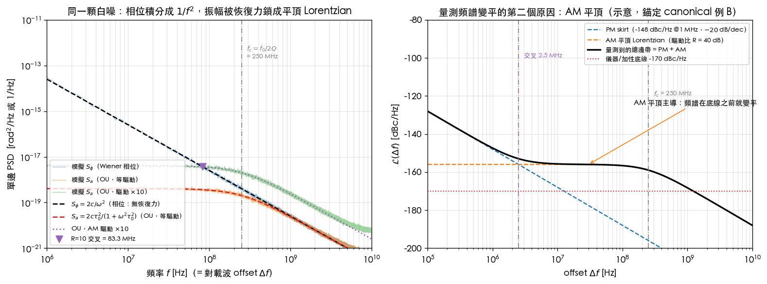
How to read it:

• Left plot: blue ($S_\phi$) follows $-20$ dB/dec all the way down; orange (equal-drive $S_a$) locks into a flat top at low frequency (measured $4.10\times10^{-19}$ /Hz vs theory $4.05\times10^{-19}$), bends at $f_c=250$ MHz (measured $-3$ dB point 239.9 MHz, about 4% low — caused by Welch segment averaging + smoothing, an estimation bias, not physics), and merges with $S_\phi$ at the high end (ratio 0.991 at 2.5 GHz vs theory 0.990). Green ($R=10$) crosses the PM skirt at 83.3 MHz (measured 83.31, theory 83.33).
• Time-domain check: the decay constant extracted from the autocorrelation, 0.6353 ns ≈ theory 0.6366 ns — this directly confirms that [P4]'s $d(t)=e^{-t/\tau_0}$ remains the backbone of the spectrum under continuous drive.
• Right plot (theory illustration, anchored to Example B): the black total sideband bends flat at 2.5 MHz, holds a $-156$ dBc/Hz plateau out to 250 MHz, then resumes $-20$ dB/dec; the red dotted line (the $-170$ dBc/Hz floor) lies further below — the flatness is not caused by the floor.
• Honesty note: (i) On the left plot, at $\gtrsim3$ GHz the simulation sits slightly above the theory line — an artifact of discretization ($\omega\,dt$ no longer $\ll1$) and aliasing, not physics. (ii) $R=40$ dB is an illustrative parameter — the actual AM/PM drive ratio is set by the topology (tail, bias, limiting strength); under equal drive AM contributes at most +3 dB to the total sideband. (iii) This simulation is a baseband-equivalent toy model (directly simulating the two slow variables $a,\phi$), not transistor-level.

5.8 Validity and failure conditions for this section

Condition	When it holds	When it fails
Small-perturbation linearization ($\lvert a\rvert\ll1$)	OU model valid	Large perturbations enter nonlinear limiting; the spectrum departs from the Lorentzian
Single amplitude decay mode, $\tau_0=2Q/\omega_0$	Corner sits exactly at $f_0/2Q$	Non-LC topologies / multiple modes have different decay rates (the general case belongs to the Floquet framework, not among the 5 source PDFs)
White-noise drive	The flat top is flat	Flicker AM superposes a $1/f$ rise inside the flat top
AM–PM ignored (Section 4)	AM and PM stay separate	AM leaks into PM via $\partial\omega/\partial A$; close-in degrades
SA measurement (collects both AM+PM)	The total-sideband formula of 5.5 applies	Phase-detector measurements reject AM; the AM flat top is invisible

Key takeaways

• The jitter that communication and clocking systems care about = a phase matter; phase has no restoring force → accumulates → $1/f^2$, $1/f^3$ skirts.
• Amplitude has a restoring force → perturbations decay exponentially (amplitude decay function $d(t-\tau)\to 0$) → bounded variance, suppressed.
• The APF $\Lambda(\omega_0\tau)$ (units $\mathrm{A^{-1}}$) is the amplitude-domain counterpart of the ISF; the phase kernel is a step $u$, the amplitude kernel is impulse × decay.
• Ideal LC: $\Gamma\propto-\sin\theta$ (tangential) and $\Lambda\propto\cos\theta$ (radial) are in quadrature (90° apart) — [P4] Fig. 5, p.2126.
• AM–PM is the back door through which amplitude noise leaks back into phase: beware when $\partial\omega/\partial A\neq 0$.
• Example A: 1 fC injected at the zero crossing → 31.8 fs of permanent jitter; at the peak → ~0 permanent effect.
• Continuous white-noise drive + exponential restoration ([P4] $\tau_0=2Q/\omega_0$) = an OU process: $S_a=c\tau_0^2/(1+\omega^2\tau_0^2)$ — a flat-top Lorentzian with corner $f_c=f_0/2Q$ ($Q=10$, 5 GHz → $\tau_0=0.64$ ns, $f_c=250$ MHz); phase, with no restoring force → $c/\omega^2$ all the way down.
• The second reason a measured spectrum flattens far out is the AM flat top (the first is the instrument/additive floor): under equal drive the asymptotes intersect exactly at $f_c$ and AM adds at most +3 dB; with stronger AM drive ($R\gt1$) the crossover is $f_x=f_c/\sqrt{R-1}$, e.g. $R=10\to83.3$ MHz. An SA measures AM+PM; phase-detector methods reject AM.
• Sources: [P4] (APF / amplitude decay / quadrature, Sec. III-D–E, Fig. 5, p.2126, verified); the phase side from [P1] Eqs.(1),(10); the OU process is standard stochastic-process mathematics (external literature, Uhlenbeck–Ornstein 1930).

Further reading

• Upstream geometry (tangential vs radial): oscillator_phase
• Exact derivation of the phase sensitivity: From impulse to phase shift — the derivation
• Why the sensitivity is periodically time-varying: LTI vs LTV
• How $c_0$ upconverts $1/f$ (the other mechanism, alongside AM–PM): flicker_upconversion
• The other close-in "flattening" (phase random walk → Lorentzian lineshape): lorentzian_linewidth
• How measurement separates AM/PM (SA vs phase detector vs cross-correlation): measurement_and_spurs
• Site-wide notation (APF $\Lambda$ registered): Unified notation table