β: This English translation is in beta — the Traditional-Chinese original is the authoritative version.

Flicker noise upconversion into 1/f³ phase noise

Prerequisites: white_noise_to_phase_noise (the same mechanism, white noise → $1/f^2$), fourier_series_of_isf (the role of the DC term $c_0$), rms_isf (the $c_0$-to-$\Gamma_{rms}$ ratio sets the corner).

Hands-on verification: this page's "symmetric vs asymmetric waveforms decide close-in $1/f^3$" simulation is in lab_07.

The previous page white_noise_to_phase_noise explained how white noise turns into $1/f^2$. But look at any real oscillator's phase-noise plot: the segment closest to the carrier is usually steeper — slope $-30$ dB/decade, i.e. $1/f^3$. Where does this steep skirt come from? Answer: device flicker noise ($1/f$ noise, the noise that is especially strong in transistors at low frequency) gets "upconverted" by the oscillator to the vicinity of the carrier.

This page answers three things: (1) what flicker noise is, (2) why only the ISF's DC term $c_0$ can upconvert it, (3) why the $1/f^3$ corner is not equal to the device's $1/f$ corner, and how waveform symmetry helps.

Physical intuition (conclusion first): low-frequency flicker noise itself lives at baseband (near DC). For it to show up near the carrier, some mechanism must "move" it up to $\omega_0$. The ISF is a periodic function, and in its Fourier series the only DC component is $c_0/2$. Only this DC term multiplies the "flicker sitting right next to DC" and gets accumulated by the phase integrator into close-in phase jitter. In other words: $c_0$ is flicker's only gate to the carrier. Push $c_0$ to 0 (via waveform symmetry) and that gate closes — the $1/f^3$ skirt drops dramatically.

Step 1: what flicker noise is, and how to model it

Flicker ($1/f$) noise is the transistor's intrinsic low-frequency noise; its PSD rises toward low frequency ($\propto 1/f$), usually attributed to carrier trapping/release at the channel–oxide interface. Below the device's $1/f$ corner $\omega_{1/f}$, flicker exceeds white noise; above it, white noise dominates. [P1] describes it with a compact model ([P1] Eq.(22), p.185):

$$\overline{i_{n,1/f}^2}=\overline{i_n^2}\cdot\frac{\omega_{1/f}}{\Delta\omega}\qquad(\Delta\omega<\omega_{1/f})$$

• How to read it: $\overline{i_n^2}$ is the white-noise floor (per-Hz); multiplied by $\omega_{1/f}/\Delta\omega$, it is amplified when $\Delta\omega<\omega_{1/f}$ and rises as $1/\Delta\omega$ — exactly the $1/f$ shape. At $\Delta\omega=\omega_{1/f}$ the two are equal (the definition of the corner).
• Unit check: $\omega_{1/f}/\Delta\omega$ is dimensionless (rad/s divided by rad/s); multiplying $\overline{i_n^2}$ ($\text{A}^2/\text{Hz}$) still gives $\text{A}^2/\text{Hz}$ ✓.
• Watch the notation: $\omega_{1/f}$ is the device $1/f$ corner (rad/s), set by the transistor process — a different thing from the phase-noise $1/f^3$ corner that appears later (see Step 4; the notation page warns about this explicitly).

Step 2: why low-frequency noise must be "upconverted" to be visible

Return to the harmonic-decomposition phase response of [P1] Eq.(13), p.183:

$$\phi(t)=\frac{1}{q_{max}}\!\left[\frac{c_0}{2}\!\int_{-\infty}^{t}\!i_n\,d\tau+\sum_{n=1}^{\infty}c_n\!\int_{-\infty}^{t}\!i_n\cos(n\omega_0\tau+\theta_n)\,d\tau\right].$$

Flicker's energy is concentrated at low frequency (near DC). Look at each term in the sum:

• Every $n\ge1$ term carries $\cos(n\omega_0\tau+\theta_n)$ — it downconverts noise sitting "right around $n\omega_0$" to baseband. But flicker has almost no energy at $n\omega_0$ ($\ge\omega_0$, which is high), so these terms cannot capture flicker.

• Only the $n=0$ (DC) term $\dfrac{c_0}{2}\int i_n\,d\tau$ has no $\cos$ multiplier — it directly integrates baseband noise. Flicker's energy is exactly at baseband, so only this term accumulates flicker into phase.

• Math used: frequency translation (mixing). $\cos(n\omega_0 t)\times$noise moves noise to $\pm n\omega_0$; only the DC multiplier ($=1$) leaves baseband noise at baseband to be integrated.

• Physical meaning (claim C4): $c_0$ (the ISF's DC Fourier coefficient) is the only channel from flicker to close-in. With $c_0=0$, flicker simply never gets up there and the $1/f^3$ skirt vanishes.

Step 3: deriving the 1/f³ phase noise (step-by-step algebra, Eq.(22)→(23))

This step "multiplies" three things together: (i) flicker injected via $c_0$, (ii) the $1/f^2$ mechanism (the integrator), (iii) and the product is $1/f^3$. No skipped steps — we compute line by line.

Step 3.1: the white-noise sum keeps only the DC term. The white-noise result (spec Section 3, formula 10; [P1] Eq.(19), p.185) is

$$\mathcal{L}\{\Delta\omega\}=10\log_{10}\!\left(\frac{(\overline{i_n^2}/\Delta f)\,\sum_{n=0}^{\infty}c_n^2}{8\,q_{max}^2\,\Delta\omega^2}\right).$$

Flicker's energy is only at baseband; from Step 2, only the $n=0$ (DC) term can capture it (the remaining $n\ge1$ terms carry $\cos(n\omega_0\tau)$, moving the noise to $n\omega_0$, where flicker has no energy). So for flicker, the sum $\sum_{n=0}^{\infty}c_n^2$ collapses to the single term $c_0^2$:

$$\sum_{n=0}^{\infty}c_n^2\ \xrightarrow{\ \text{flicker 只剩 DC}\ }\ c_0^2.$$

• Why this $c_0^2$ pairs with the $8$ in the denominator: Eq.(19)'s denominator is $8q_{max}^2\Delta\omega^2$ and its numerator carries $\sum c_n^2$. The DC term of the ISF Fourier series ([P1] Eq.(12)) is written $\tfrac{c_0}{2}$, but in Parseval ([P1] Eq.(20)) the DC power coefficient is recorded as $c_0^2$ (the same convention as the other $c_n^2$), so we substitute $c_0^2$ directly and keep the $8$ in the denominator. Substituting gives the "DC-only, still white-noise" intermediate form:

$$\mathcal{L}\{\Delta\omega\}\Big|_{1/f^2,\,\text{DC only}}=10\log_{10}\!\left(\frac{c_0^2}{q_{max}^2}\cdot\frac{\overline{i_n^2}/\Delta f}{8\,\Delta\omega^2}\right).$$

Step 3.2: replace the white-noise floor with flicker (multiply by the amplification factor of Eq.(22)). The $\overline{i_n^2}/\Delta f$ in the numerator above is still the white-noise floor. Device flicker ([P1] Eq.(22), p.185) says that for $\Delta\omega<\omega_{1/f}$, the current noise is amplified by $\omega_{1/f}/\Delta\omega$:

$$\overline{i_{n,1/f}^2}=\overline{i_n^2}\cdot\frac{\omega_{1/f}}{\Delta\omega}.$$

Replacing the numerator's $\overline{i_n^2}/\Delta f$ with $\overline{i_{n,1/f}^2}/\Delta f=(\overline{i_n^2}/\Delta f)\cdot(\omega_{1/f}/\Delta\omega)$ is exactly the product "flicker mechanism × $1/f^2$ mechanism":

$$\frac{c_0^2}{q_{max}^2}\cdot\underbrace{\frac{\overline{i_n^2}/\Delta f}{8\,\Delta\omega^2}}_{1/f^2\ \text{機制（積分器）}}\;\times\;\underbrace{\frac{\omega_{1/f}}{\Delta\omega}}_{\text{flicker 機制}}.$$

Step 3.3: combine to get [P1] Eq.(23). Multiplying the two brackets and putting back the $10\log_{10}$ yields the flicker-upconverted $1/f^3$ phase noise ([P1] Eq.(23), p.185):

$$\boxed{\ \mathcal{L}\{\Delta\omega\}=10\log_{10}\!\left(\frac{c_0^2}{q_{max}^2}\cdot\frac{\overline{i_n^2}/\Delta f}{8\,\Delta\omega^2}\cdot\frac{\omega_{1/f}}{\Delta\omega}\right)\ }$$

• See the $1/f^3$? The denominator has $\Delta\omega^2$ (the integrator, $1/f^2$) times one more $\Delta\omega$ (flicker's $1/\Delta\omega$), together $\Delta\omega^3$. One decade up drops it $1000$× $\Rightarrow 30$ dB $\Rightarrow$ slope $-30$ dB/decade ✓.
• Key contrast: the white-noise result carries $\Gamma_{rms}^2$ (all harmonics, $=\tfrac12\sum c_n^2$); the flicker result carries $c_0^2$ (DC only). This is the mathematical root of "symmetry can only save flicker, not white noise" — in Step 4, dividing these two numerators directly yields the corner.
• Unit check: relative to the white-noise formula we multiplied by the dimensionless $\omega_{1/f}/\Delta\omega$ (rad/s ÷ rad/s); dimensions unchanged, still per-Hz ✓.

Step 4: the 1/f³ corner (Eq.(24)) — it is not the device 1/f corner

On the phase-noise spectrum, the offset where the $1/f^3$ segment meets the $1/f^2$ segment is called the $1/f^3$ corner $\Delta\omega_{1/f^3}$. Set the $1/f^3$ expression (Eq.(23), with $c_0^2$) equal to the $1/f^2$ expression (Eq.(21), with $\Gamma_{rms}^2$) and solve for the intersection ([P1] Eq.(24), p.185):

$$\boxed{\ \Delta\omega_{1/f^3}=\omega_{1/f}\cdot\frac{c_0^2}{2\,\Gamma_{rms}^2}\approx\omega_{1/f}\left(\frac{c_0}{c_1}\right)^2\ }$$

Step-by-step algebra (solving for the intersection, no skipped steps): the corner is defined as the $\Delta\omega$ where "$1/f^3$ segment = $1/f^2$ segment". Set the two brackets inside the $\log_{10}$ equal (equal logs ⇔ equal arguments):

$$\underbrace{\frac{c_0^2}{q_{max}^2}\cdot\frac{\overline{i_n^2}/\Delta f}{8\,\Delta\omega^2}\cdot\frac{\omega_{1/f}}{\Delta\omega}}_{\text{Eq.(23)：}1/f^3} =\underbrace{\frac{\Gamma_{rms}^2}{q_{max}^2}\cdot\frac{\overline{i_n^2}/\Delta f}{4\,\Delta\omega^2}}_{\text{Eq.(21)：}1/f^2}.$$

• Step (a): cancel the common factors. Both sides carry $\dfrac{1}{q_{max}^2}$ and $\dfrac{\overline{i_n^2}/\Delta f}{\Delta\omega^2}$; divide them out:

$$\frac{c_0^2}{8}\cdot\frac{\omega_{1/f}}{\Delta\omega}=\frac{\Gamma_{rms}^2}{4}.$$

• Step (b): solve for $\Delta\omega$. Multiply both sides by $\Delta\omega$, then divide by $\Gamma_{rms}^2/4$:

$$\frac{c_0^2\,\omega_{1/f}}{8}=\frac{\Gamma_{rms}^2}{4}\,\Delta\omega \;\Longrightarrow\; \Delta\omega=\frac{c_0^2\,\omega_{1/f}}{8}\cdot\frac{4}{\Gamma_{rms}^2}=\omega_{1/f}\cdot\frac{4c_0^2}{8\,\Gamma_{rms}^2}=\omega_{1/f}\cdot\frac{c_0^2}{2\,\Gamma_{rms}^2}.$$

$4/8=1/2$, giving exactly the boxed $\dfrac{c_0^2}{2\Gamma_{rms}^2}$ ✓. Note the factor here is $\tfrac12$ (not $\tfrac14$); it comes from the ratio of the $8$ in Eq.(23)'s denominator to the $4$ in Eq.(21)'s denominator.

• The most important concept on this page (claim C5): $\Delta\omega_{1/f^3}\ne\omega_{1/f}$. The $1/f^3$ corner equals the device's $1/f$ corner times the ratio $c_0^2/(2\Gamma_{rms}^2)$. Because a symmetric waveform has $c_0\ll\Gamma_{rms}$, this ratio is far below 1, so the $1/f^3$ corner is pushed far below the device's $1/f$ corner. This overturns the myth of the early empirical model "$1/f^3$ corner $=$ device $1/f$ corner" — [P1]'s abstract and introduction emphasize that "contrary to widely held beliefs, the $1/f^3$ corner is smaller than the device $1/f$ corner by a factor determined by waveform symmetry".
• Where $\approx\omega_{1/f}(c_0/c_1)^2$ comes from: when the ISF is fundamental-dominated, $\Gamma_{rms}^2\approx c_1^2/2$ (Parseval keeps only the $n=1$ term); substituting gives the right-hand form. It lets you estimate the corner directly from "DC coefficient vs fundamental coefficient".
• Unit check: $\omega_{1/f}$ (rad/s) times a dimensionless ratio → rad/s ✓, an angular frequency.

Step 5: why waveform symmetry determines $c_0$

$c_0$ is the ISF's DC Fourier coefficient; the ISF's DC value is $c_0/2$ (the notation trap flagged on the notation page). The DC value is the ISF's average over one period. [P1] points out in the design section (p.187–188, Fig. 16):

The DC value of the ISF is determined by the waveform's symmetry, in particular its rise/fall symmetry. If the rise time and fall time differ significantly, the ISF has a large DC value (large $c_0$).

Intuition: the ISF swings positive and negative in the "sensitive region" (near the waveform transitions). If the rising and falling segments are mirror-symmetric, the positive and negative swings cancel and the average $\approx0$ (small $c_0$); if they are asymmetric (e.g. fast rise, slow fall), they do not cancel, the average is nonzero (large $c_0$), and flicker's gate opens wide.

• Odd-symmetric waveforms (odd-symmetric, e.g. an ideal $-\sin$, antiphase over half a period) have $c_0=0$ — an excellent special case; but [P1] clarifies explicitly: small $c_0$ is not limited to odd-symmetric waveforms — rise/fall symmetry alone suffices, a much broader class.
• Toy contrast: lab_05 uses $\Gamma=\cos\theta$ (symmetric, $c_0=0$) against $\Gamma=\cos\theta+0.4$ (deliberately added DC, $c_0=0.8$) to show directly whether the DC term is present.

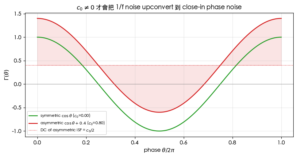
Waveform	ISF DC value $c_0/2$	$c_0$	Flicker upconversion
Symmetric ($\cos\theta$, rise=fall)	$0$	$0$	almost no $1/f^3$
Asymmetric ($\cos\theta+0.4$)	$0.4$	$0.8$	pronounced $1/f^3$ skirt

Step 6: how differential / complementary waveforms help — and their limits

In practice two tricks are commonly used to approach symmetry and suppress $c_0$:

• Differential: use a pair of complementary nodes to cancel even harmonics and common-mode error, improving symmetry.
• Complementary (complementary CMOS, symmetric PMOS/NMOS arrangement): deliberately match pull-up/pull-down so that rise/fall times are equal → rise/fall symmetry → small $c_0$.

[P2] (the ring-oscillator paper) confirms this rule directly by experiment: phase noise varies with the "symmetry control voltage" and reaches a minimum at the symmetry point, and the $1/f^3$ corner drops sharply at the symmetry point ([P2] Fig. 17, p.802; corresponds to claim C4).

Limits (honesty note) — [P2] also points out (Sec. VII Design Implications, p.798, original text):

• Differential symmetry is not necessarily enough: [P2] states plainly that "differential symmetry is insufficient"; what is needed is rise/fall symmetry within each half period, not merely symmetry between the two differential branches.
• The tail / bias source is a major leak: the ISF of the tail current source often has a large DC value, strongly upconverting the tail's flicker, which frequently dominates close-in noise. Symmetrizing the main signal path does not help — the tail must be handled separately.
• More linear loads help: [P2] recommends more linear loads (e.g. resistors or long-channel devices) to make the waveform more symmetric and push the corner further down.
• Even so, symmetry only suppresses flicker ($1/f^3$); it does not change the white-noise $1/f^2$ region (that region is set by $\Gamma_{rms}$, not $c_0$). Do not expect symmetry to rescue the whole curve.

Numerical example (building intuition)

Continuing Example B: $f_0=5$ GHz, $q_{max}=1$ pC, $\Gamma_{rms}=0.5$. Assume a device $1/f$ corner $f_{1/f}=1$ MHz ($\omega_{1/f}=2\pi\times10^6$ rad/s). Compare the $1/f^3$ corner for a symmetric ($c_0=0.04$) and an asymmetric ($c_0=0.4$) waveform.

Using [P1] Eq.(24): $\Delta\omega_{1/f^3}=\omega_{1/f}\cdot c_0^2/(2\Gamma_{rms}^2)$, $2\Gamma_{rms}^2=2\times0.25=0.5$.

Asymmetric ($c_0=0.4$, $c_0^2=0.16$):

$$\frac{f_{1/f^3}}{f_{1/f}}=\frac{c_0^2}{2\Gamma_{rms}^2}=\frac{0.16}{0.5}=0.32\;\Rightarrow\;f_{1/f^3}=0.32\times1\,\text{MHz}=320\ \text{kHz}.$$

Symmetric ($c_0=0.04$, $c_0^2=1.6\times10^{-3}$):

$$\frac{f_{1/f^3}}{f_{1/f}}=\frac{1.6\times10^{-3}}{0.5}=3.2\times10^{-3}\;\Rightarrow\;f_{1/f^3}=3.2\times10^{-3}\times1\,\text{MHz}=3.2\ \text{kHz}.$$

• Feel for it: the device $1/f$ corner is 1 MHz in both cases, but the phase-noise $1/f^3$ corner drops from 320 kHz (asymmetric) to 3.2 kHz (symmetric) — a full 100× lower (because $c_0^2$ differs by 100×). This is the numerical picture of "$1/f^3$ corner ≠ device $1/f$ corner": good symmetry pushes the steep skirt in very close to the carrier, leaving the close-in region much cleaner.
• Dimension check: the corner is a frequency; $\text{MHz}\times$ (dimensionless ratio) $=$ frequency ✓.

Corresponding simulation plot (toy model, not transistor-level)

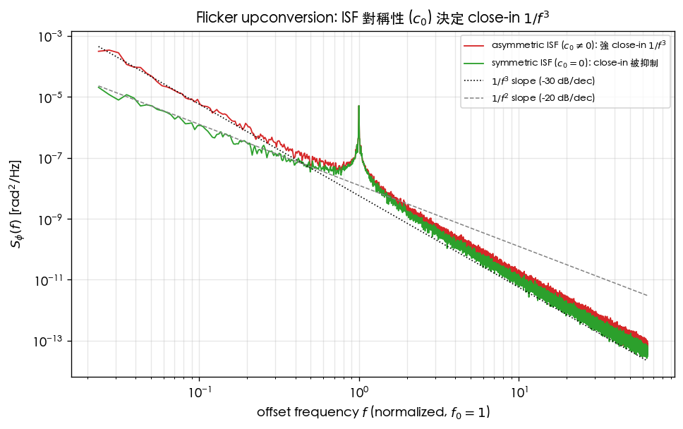
lab_07 feeds flicker current into a symmetric ($\cos$, $c_0=0$) and an asymmetric ($\cos+0.5$) toy ISF and estimates the close-in phase PSD: the symmetric case shows almost no $1/f^3$, while the asymmetric case shows a clear $-30$ dB/decade skirt. For a visualization of $c_0$ see lab_05's symmetric_vs_asymmetric_isf_c0.png (table above).

Core Python (full script: simulations/lab_07_flicker_noise.py):

import numpy as np
from simulations.common.noise_utils import flicker_noise, estimate_psd
from simulations.common.isf_utils import gamma_symmetric, gamma_asymmetric

fs, n, qmax = 256.0, 2**20, 1.0
t = np.arange(n) / fs
theta = 2 * np.pi * 1.0 * t                          # f0 = 1 (toy normalized frequency)

i_f = flicker_noise(n, fs, k_flicker=1e-4)           # 1/f current

# ISF weighting + integrator: phi = cumsum(Gamma * i_n / qmax) / fs
def phase_from_isf(i_n, gamma_vals, q_max, fs):
    g = gamma_vals * i_n / q_max
    return np.cumsum(g) / fs

gamma_sym  = gamma_symmetric(theta)                  # c0 = 0
gamma_asym = gamma_asymmetric(theta, alpha=0.5)      # c0 = 2*alpha = 1.0 (DC = 0.5)

phi_sym  = phase_from_isf(i_f, gamma_sym,  qmax, fs)  # symmetric -> close-in nearly flat
phi_asym = phase_from_isf(i_f, gamma_asym, qmax, fs)  # asymmetric -> 1/f^3 skirt

Applicability and failure conditions

Condition	When it holds	What happens when it fails
$\Delta\omega<\omega_{1/f}$	flicker model (Eq.22) holds, giving $1/f^3$	above the corner it reverts to white-noise $1/f^2$
Small perturbation, phase linearity	Eq.(13) harmonic-decomposition form holds	large injection → ISF distorts, $c_0$ changes
Correct $c_0$ known	corner prediction accurate	$c_0$ is very sensitive to waveform detail, tail, load; extract by simulation
Symmetrized main path	effective at suppressing $1/f^3$	no effect on tail flicker or white-noise $1/f^2$

Which papers / equations this maps to

• Device flicker model [P1] Eq.(22), p.185; $1/f^3$ phase noise [P1] Eq.(23), p.185; $1/f^3$ corner [P1] Eq.(24), p.185.
• Upstream harmonic-decomposition form [P1] Eq.(13), p.183; symmetry design discussion [P1] Sec. IV & Fig. 16, p.187–188.
• Experimental evidence for symmetry [P2] Fig. 17, p.802; limits of differential symmetry [P2] Sec. VII (Design Implications), p.798.
• Claims C4 (only $c_0$ upconverts; symmetry suppresses it) and C5 (corner ≠ device corner).

Worked examples

Both problems use the exact form of [P1] Eq.(24): $\Delta\omega_{1/f^3}=\omega_{1/f}\cdot\dfrac{c_0^2}{2\Gamma_{rms}^2}$. We keep the site-wide canonical $\Gamma_{rms}=0.5$ (so $2\Gamma_{rms}^2=0.5$) and plug in two sets of $c_0,\omega_{1/f}$. Special case: if the ISF contains only the fundamental ($c_1\gg c_2,c_3,\dots$), Parseval ([P1] Eq.(20)) gives $\Gamma_{rms}^2=c_1^2/2$, and the exact form reduces to $\dfrac{c_0^2}{2\Gamma_{rms}^2}=\dfrac{c_0^2}{c_1^2}=(c_0/c_1)^2$; this page uses the exact form for the numbers, not this special case. Format: problem → step-by-step substitution (with units) → result → dimension check → one-line Python verification.

Example E: 1/f³ corner of an asymmetric waveform (large $c_0$)

Problem: $c_0=0.4$, canonical $\Gamma_{rms}=0.5$, device $f_{1/f}=1$ MHz ($\omega_{1/f}=2\pi\times10^6$ rad/s). Find the phase-noise $1/f^3$ corner $f_{1/f^3}$.

Step 1 (compute the ratio $c_0^2/(2\Gamma_{rms}^2)$): $\dfrac{c_0^2}{2\Gamma_{rms}^2}=\dfrac{0.4^2}{2\times0.5^2}=\dfrac{0.16}{0.5}=0.32$ (dimensionless).

Step 2 (multiply by the device corner): the corner is a frequency, so we can work directly in Hz (the $2\pi$ cancels in the ratio):

$$f_{1/f^3}=f_{1/f}\cdot\frac{c_0^2}{2\Gamma_{rms}^2}=1\,\text{MHz}\times0.32=320\ \text{kHz}.$$

• Result: $f_{1/f^3}=320$ kHz, already below the device's 1 MHz corner — even for this "not particularly symmetric" waveform, the $1/f^3$ corner is already pushed below the device corner (because $c_0\ll\Gamma_{rms}\cdot\sqrt2$). This value is consistent with symmetry and device_noise_mapping.
• Dimension check: $f_{1/f}$ (Hz) × dimensionless ratio = Hz ✓, a frequency.

from simulations.common.isf_utils import gamma_rms  # noqa: F401
# corner set by the exact form c0^2/(2*Gamma_rms^2) (Eq.24); canonical Gamma_rms=0.5
c0, gamma_rms_val, f_1f = 0.4, 0.5, 1e6
f_1f3 = f_1f * c0**2 / (2*gamma_rms_val**2)
print(f_1f3/1e3, "kHz")          # -> 320.0 kHz

Example F: how symmetrization (small $c_0$) pushes the corner down

Problem: symmetrize the waveform of Example E so that $c_0$ drops from 0.4 to 0.04 (canonical $\Gamma_{rms}=0.5$ and $f_{1/f}=1$ MHz unchanged). Find the new $f_{1/f^3}$ and explain how symmetry does its work.

Step 1 (new ratio): $\dfrac{c_0^2}{2\Gamma_{rms}^2}=\dfrac{0.04^2}{2\times0.5^2}=\dfrac{1.6\times10^{-3}}{0.5}=3.2\times10^{-3}$.

Step 2 (multiply by the device corner):

$$f_{1/f^3}=1\,\text{MHz}\times3.2\times10^{-3}=3.2\ \text{kHz}.$$

• Result: $f_{1/f^3}=3.2$ kHz. A 10× drop in $c_0$ $\Rightarrow$ a 100× drop in $c_0^2$ $\Rightarrow$ the corner falls from 320 kHz to 3.2 kHz (100× lower).
• How symmetry pushes it down (the point of this problem): corner $\propto c_0^2$, and $c_0/2$ is the ISF's average over one period (the DC value). Make the waveform's rise/fall symmetric, and the ISF's positive and negative swings in the sensitive region cancel → $c_0$ approaches 0 → the corner collapses at a quadratic rate. This is the numerical picture of "$1/f^3$ corner ≠ device $1/f$ corner": the device corner is still 1 MHz, but the steep close-in skirt is pushed down to 3.2 kHz, leaving the carrier's vicinity much cleaner.
• Dimension check: Hz × dimensionless = Hz ✓.

# symmetrization shrinks c0 -> corner ∝ c0^2 collapses quadratically (canonical Gamma_rms=0.5)
f_1f = 1e6; gamma_rms_val = 0.5
for c0 in (0.4, 0.04):
    print(c0, "->", f_1f*c0**2/(2*gamma_rms_val**2)/1e3, "kHz")   # 0.4 -> 320.0 kHz ; 0.04 -> 3.2 kHz

Key takeaways

• Flicker is the device's low-frequency noise ($\propto1/f$); it must be "upconverted" to appear near the carrier.
• Only the ISF's DC term $c_0$ can upconvert flicker → close-in becomes $-30$ dB/decade $1/f^3$ (Eq.23).
• $1/f^3$ corner $=\omega_{1/f}\cdot c_0^2/(2\Gamma_{rms}^2)\ne$ device $1/f$ corner (Eq.24); a symmetric waveform (small $c_0$) pushes the corner far below the device corner.
• Waveform rise/fall symmetry $\Rightarrow$ ISF average ($c_0/2$) $\approx0$ $\Rightarrow$ $1/f^3$ drops dramatically.
• Differential/complementary designs help symmetry, but differential symmetry alone is not enough, the tail source's large $c_0$ is a leak, and symmetry does not improve the white-noise $1/f^2$ region.
• Numbers: with a 1 MHz device corner and canonical $\Gamma_{rms}=0.5$, moving $c_0$ from 0.4→0.04 takes the $1/f^3$ corner from 320 kHz→3.2 kHz (a factor of 100).

Further reading

• The white-noise region: white_noise_to_phase_noise
• ISF Fourier series and $c_0$: fourier_series_of_isf
• Cyclostationary noise and tail gating: effective_isf
• Dedicated symmetry design page: symmetry
• Simulation verification: lab_07, lab_05