The rms ISF and the Parseval Relation

β: This English translation is in beta — the Traditional-Chinese original is the authoritative version.

Prerequisites: fourier_series_of_isf (the $c_n$ coefficients of $\Gamma$), stochastic_noise_basics (Parseval / power spectra), convolution_derivation (the phase integral).

The previous page, fourier_series_of_isf, decomposed the ISF into a set of Fourier coefficients $c_0,c_1,c_2,\dots$ and showed that each $c_n$ folds the noise near $n\omega_0$ back onto the carrier. This page answers:

When the device noise is flat white noise and the contributions of all bands must be summed, can a single number describe the entire ISF's contribution to phase noise? It can — that number is the rms value of the ISF, $\Gamma_{rms}$, tied to the sum of squared coefficients by Parseval's theorem ([P1] Eq.(20), p.185):

$$\sum_{n=0}^{\infty}c_n^2=\frac{1}{\pi}\int_0^{2\pi}|\Gamma(x)|^2dx=2\,\Gamma_{rms}^2$$

Physical intuition (conclusion first): white noise is equally strong in every $n\omega_0$ band, so the "total folded-back power" is proportional to the sum of the squares of all coefficients, $\sum c_n^2$. Parseval tells us this sum equals twice the mean square of the ISF over one period, i.e. $2\Gamma_{rms}^2$. The messy band-by-band summation thus collapses into one clean shape metric, $\Gamma_{rms}$ — which (together with $q_{max}$) sets the level of the $1/f^2$ phase noise. Intuitively: the "quieter" the ISF is overall (the smaller its rms), the less sensitive the oscillator is to white noise.

Step 1: Parseval's theorem — time-domain energy = sum of squared frequency-domain coefficients

Parseval's theorem states: the mean square of a periodic function over one period equals the sum of the mean squares of its Fourier components. For the standard cos/sin expansion $\Gamma(x)=\dfrac{a_0}{2}+\sum_{n\ge1}[a_n\cos nx+b_n\sin nx]$:

$$\frac{1}{2\pi}\int_0^{2\pi}|\Gamma(x)|^2\,dx =\left(\frac{a_0}{2}\right)^2+\frac{1}{2}\sum_{n=1}^{\infty}(a_n^2+b_n^2).$$

• Math used: the basis $\{1,\cos nx,\sin nx\}$ is orthogonal. After expanding $|\Gamma|^2$, all cross terms such as $\int\cos mx\cos nx\,dx$ ($m\neq n$) integrate to 0; only the "self-with-self" terms survive.
• Where each term's coefficient comes from: $\dfrac{1}{2\pi}\int_0^{2\pi}\cos^2(nx)\,dx=\dfrac12$ ($n\ge1$), so each $a_n\cos nx$ contributes $\dfrac12 a_n^2$ to the mean square; the constant term $\dfrac{a_0}{2}$ has mean square $\left(\dfrac{a_0}{2}\right)^2$ (the mean square of a constant is its own square — no $\frac12$). This factor difference between the DC and AC terms is the single most error-prone spot in the entire derivation; Step 4 is devoted to it.

Step-by-step algebra (killing the cross terms one at a time, no skipped steps): first expand the square of $\Gamma$ in full, then integrate class by class.

$$\begin{aligned} \frac{1}{2\pi}\int_0^{2\pi}|\Gamma|^2dx &=\frac{1}{2\pi}\int_0^{2\pi}\!\left[\frac{a_0}{2}+\sum_{m\ge1}(a_m\cos mx+b_m\sin mx)\right]^2 dx\\ &=\underbrace{\frac{1}{2\pi}\int_0^{2\pi}\left(\frac{a_0}{2}\right)^2 dx}_{\text{(I) DC×DC}} +\underbrace{\frac{1}{2\pi}\int_0^{2\pi}2\cdot\frac{a_0}{2}\sum_{m\ge1}(a_m\cos mx+b_m\sin mx)\,dx}_{\text{(II) DC×AC}}\\ &\quad+\underbrace{\frac{1}{2\pi}\int_0^{2\pi}\Big[\sum_{m\ge1}(a_m\cos mx+b_m\sin mx)\Big]^2 dx}_{\text{(III) AC×AC}}. \end{aligned}$$

Term by term (with the orthogonality used at each step called out):

• (I): the integrand is a constant, $\dfrac{1}{2\pi}\int_0^{2\pi}\left(\dfrac{a_0}{2}\right)^2dx=\left(\dfrac{a_0}{2}\right)^2$.
• (II): every $\int_0^{2\pi}\cos mx\,dx=\int_0^{2\pi}\sin mx\,dx=0$ ($m\ge1$), so the whole block = 0. This is "the constant is orthogonal to every harmonic."
• (III): expanding the square produces three kinds of integrals. First, $\int_0^{2\pi}\cos mx\cos nx\,dx=\pi\,\delta_{mn}$ and $\int_0^{2\pi}\sin mx\sin nx\,dx=\pi\,\delta_{mn}$ ($m,n\ge1$); second, $\int_0^{2\pi}\cos mx\sin nx\,dx=0$ (all of these vanish — cos and sin are mutually orthogonal). Only the $m=n$ "self-with-self" terms survive, each weighted $\dfrac{1}{2\pi}\cdot\pi=\dfrac12$:

$$\text{(III)}=\frac12\sum_{n\ge1}(a_n^2+b_n^2).$$

Collecting (I)+(II)+(III) recovers the line above, $\left(\frac{a_0}{2}\right)^2+\frac12\sum_{n\ge1}(a_n^2+b_n^2)$. The soul of the whole passage is one sentence: the basis is orthogonal, so the squared integral keeps only the "diagonal" terms.

Step 2: switching to the amplitude–phase coefficients $c_n$

Use the correspondence from the previous page: $c_n^2=a_n^2+b_n^2$ ($n\ge1$), and the DC coefficient $c_0\equiv a_0$. Substituting into Step 1:

$$\frac{1}{2\pi}\int_0^{2\pi}|\Gamma|^2\,dx =\left(\frac{c_0}{2}\right)^2+\frac12\sum_{n=1}^{\infty}c_n^2 =\frac{c_0^2}{4}+\frac12\sum_{n=1}^{\infty}c_n^2.$$

• Simplification trick: note that $\dfrac{c_0^2}{4}=\dfrac12\cdot\dfrac{c_0^2}{2}$. To fold DC into the same summation, Hajimiri–Lee adopt the bookkeeping "$c_0$ carries half weight inside the sum" — i.e. the $n=0$ term contributes $\dfrac12\cdot\dfrac{c_0^2}{2}$. The next step shows this is exactly what lets the total be written in its cleanest form.

Step 3: arriving at [P1] Eq.(20) — defining $\Gamma_{rms}$

Multiply both sides of Step 2 by 2:

$$\frac{1}{\pi}\int_0^{2\pi}|\Gamma|^2\,dx =\frac{c_0^2}{2}+\sum_{n=1}^{\infty}c_n^2.$$

In [P1] Eq.(20), Hajimiri–Lee define the left side as $2\Gamma_{rms}^2$ and write the right side as $\sum_{n=0}^{\infty}c_n^2$ — i.e. by convention the $n=0$ term inside the sum stands for $\dfrac{c_0^2}{2}$ (not $c_0^2$). This yields the signature equation at the top of this page:

$$\boxed{\ \sum_{n=0}^{\infty}c_n^2=\frac{1}{\pi}\int_0^{2\pi}|\Gamma(x)|^2dx=2\,\Gamma_{rms}^2\ }\qquad[\text{P1] Eq.(20), p.185}$$

where $\Gamma_{rms}$ is simply the root-mean-square of the ISF:

$$\Gamma_{rms}=\sqrt{\frac{1}{2\pi}\int_0^{2\pi}|\Gamma(x)|^2\,dx}.$$

• Dimension check: $\Gamma$ is dimensionless ⟹ $|\Gamma|^2$ is dimensionless ⟹ dividing the integral by $2\pi$ (rad) and taking the square root leaves it dimensionless ✓. $c_n$ is dimensionless too, so both sides agree.
• This site's Python: gamma_rms(theta, gamma) computes exactly $\sqrt{\frac{1}{2\pi}\int_0^{2\pi}\Gamma^2}$ (see the simulations/common/isf_utils.py docstring, explicitly matched to Eq.(20)).

Step 4: teaching note on the DC-term factor (the most error-prone spot)

Read this section carefully — otherwise you will be off by a factor when computing the $1/f^3$ corner ([P1] Eq.(24)). Keep the three flavors of "$c_0$" straight:

Name	Expression	Appears in
the ISF's DC value (its mean)	$\dfrac{c_0}{2}$	the constant term in Eq.(12); the single-tone response in Eq.(15)
the Fourier DC coefficient	$c_0$ ($=a_0=\frac{1}{\pi}\int_0^{2\pi}\Gamma\,dx$)	the bar chart; the $n=0$ term of Eq.(20)
the $n=0$ contribution in the Parseval sum	$\dfrac{c_0^2}{2}$ (not $c_0^2$!)	the right side of Eq.(20), $\sum_{n=0}^\infty c_n^2$

• Why DC enters the sum at "half weight": an AC harmonic $c_n\cos(nx+\theta_n)$ has mean square $\dfrac12 c_n^2$ (the time average of cosine, $\langle\cos^2\rangle=\frac12$); but DC is a constant, whose mean square is $\left(\dfrac{c_0}{2}\right)^2 =\dfrac{c_0^2}{4}$. For "multiply by 2 and write it as $\sum_{n\ge0}c_n^2$" to be formally consistent for every $n$, the $n=0$ term must count only $\dfrac{c_0^2}{2}$ (i.e. treat $c_0$ as "half a coefficient" in the rms sum).
• Teaching reminder: many textbooks (and the notation traps in this site's notation) hammer this point — $c_0$ is the "coefficient"; the DC "value" is $c_0/2$. The constants in the phase-noise formulas (e.g. $c_0^2/8$ in Eq.(23), $c_0^2/(2\Gamma_{rms}^2)$ in Eq.(24)) are exactly this factor carried all the way through. Copy the equations from Section 3 of the spec verbatim — do not re-insert factors yourself — and you will not go wrong.

Step 5: how $\Gamma_{rms}$ sets the $1/f^2$ phase noise

Substitute Eq.(20) into the white-noise phase-noise summation ([P1] Eq.(19), p.185):

$$\mathcal{L}\{\Delta\omega\}=10\log_{10}\!\left(\frac{\overline{i_n^2}/\Delta f\;\sum_{n=0}^{\infty}c_n^2}{8\,q_{max}^2\,\Delta\omega^2}\right).$$

Using $\sum_{n=0}^{\infty}c_n^2=2\Gamma_{rms}^2$ to replace $\sum c_n^2$, the $8$ in the denominator and the $2$ in the numerator reduce to $4$, giving the signature result ([P1] Eq.(21), p.185):

$$\mathcal{L}\{\Delta\omega\}=10\log_{10}\!\left(\frac{\Gamma_{rms}^2}{q_{max}^2}\cdot\frac{\overline{i_n^2}/\Delta f}{4\,\Delta\omega^2}\right).$$

• How to read it: phase noise is proportional to $\dfrac{\Gamma_{rms}^2}{q_{max}^2}$ and falls with offset $\Delta\omega$ as $1/\Delta\omega^2$ (i.e. $-20$ dB/dec, the $1/f^2$ region). Two design knobs: increase $q_{max}$ (the signal charge swing) and shrink $\Gamma_{rms}$ (keep the ISF quiet overall).
• Factor-of-2 teaching note: a clean time-domain "white noise × ISF → integrate" derivation gives $S_\phi(f)=\Gamma_{rms}^2 S_i/(q_{max}^2(2\pi f)^2)$, corresponding to $\mathcal{L}=\Gamma_{rms}^2 S_i/(2q_{max}^2\Delta\omega^2)$; [P1] Eq.(21) writes $/(4\Delta\omega^2)$. The factor of 2 comes from the SSB (single-sideband) bookkeeping convention — a well-known small dispute in the literature — and does not affect the $\Gamma_{rms}^2/q_{max}^2$ scaling or the $-20$ dB/dec slope. Full discussion in white_noise_to_phase_noise.

Numerical examples (building a feel)

Example 1: $\Gamma_{rms}$ of the ideal LC (two methods cross-checked)

Take $\Gamma(\theta)=-\sin\theta$.

Method A (integral):

$$\Gamma_{rms}^2=\frac{1}{2\pi}\int_0^{2\pi}\sin^2\theta\,d\theta=\frac{1}{2\pi}\cdot\pi=\frac12 \ \Rightarrow\ \Gamma_{rms}=\frac{1}{\sqrt2}\approx0.707.$$

Method B (coefficients): the previous page gave $c_0=0,\ c_1=1$, all others 0. By Eq.(20), $\sum c_n^2=c_1^2=1=2\Gamma_{rms}^2$ ⟹ $\Gamma_{rms}=1/\sqrt2\approx0.707$. The two agree ✓.

• Feel: $\Gamma_{rms}\approx0.707$ is the benchmark value for a "clean single-tone ISF". This site's canonical worked example (Example B) uses $\Gamma_{rms}=0.5$ as the representative value — slightly below the ideal $-\sin$, corresponding to an ISF somewhat flattened by factors other than $q_{max}$.

Example 2: $1/f^2$ phase noise with $\Gamma_{rms}=0.5$ (canonical Example B)

$f_0=5$ GHz, $\Delta f=1$ MHz, $q_{max}=1$ pC, $\Gamma_{rms}=0.5$, $S_i=10^{-24}$ A²/Hz.

First compute $\Delta\omega=2\pi\times10^6=6.283\times10^6$ rad/s, $\Delta\omega^2=3.948\times10^{13}$. Use Eq.(21) (i.e. the SSB $/(4\Delta\omega^2)$ convention — see the factor-of-2 note in Step 5; the clean time-domain $/(2\Delta\omega^2)$ version would come out 3 dB higher):

$$\mathcal{L}=10\log_{10}\!\left[\frac{0.25}{10^{-24}}\cdot\frac{10^{-24}}{4\times3.948\times10^{13}}\right] =10\log_{10}\!\left[\frac{0.25}{4\times3.948\times10^{13}}\right].$$

The bracket $=\dfrac{0.25}{1.579\times10^{14}}=1.583\times10^{-15}$, so

$$\mathcal{L}=10\log_{10}(1.583\times10^{-15})\approx-148.0\ \text{dBc/Hz}.$$

• Dimension check: $\dfrac{\Gamma_{rms}^2}{q_{max}^2}\cdot\dfrac{S_i}{\Delta\omega^2} =\dfrac{1}{[\text{C}]^2}\cdot\dfrac{[\text{A}^2/\text{Hz}]}{[\text{rad/s}]^2}$; since $\text{C}=\text{A}\cdot\text{s}$, $\text{Hz}=1/\text{s}$, and rad is dimensionless, this reduces to $\dfrac{\text{A}^2\cdot\text{s}}{\text{A}^2\text{s}^2}\cdot\text{s}=$ dimensionless (the per-Hz is already included); after the $\log$, dBc/Hz ✓.
• Feel: this is the number for a "single ideal white-noise source"; a real circuit has multiple sources, cyclostationarity, and flicker, and will come out higher (worse). Full derivation in white_noise_to_phase_noise.

Figure 1: verifying $\sum c_n^2=2\Gamma_{rms}^2$ with the coefficient spectrum

The figure below (fig_coefficients from lab_05, n_harmonics=8) plots the $c_n$ as a bar chart and compares, on the plot, "$\sum_{n=0}^{\infty}c_n^2$ (computed on the coefficient side)" against "$2\Gamma_{rms}^2$ (computed on the integral side)" — they match, which is precisely the numerical verification of Parseval ([P1] Eq.(20)).

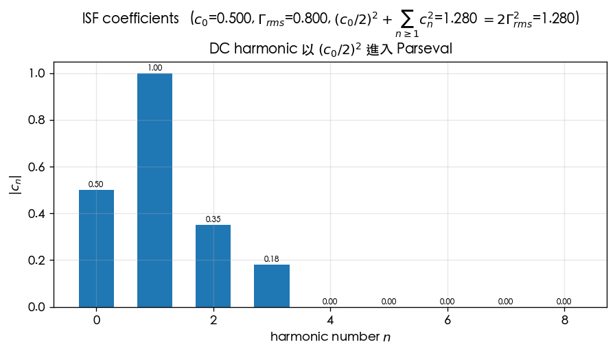
• Matching equation: [P1] Eq.(20).
• How to read it: square each bar's height and add them up (remember the $n=0$ bar counts at "half weight", $c_0^2/2$) — the total equals $2\Gamma_{rms}^2$. This gives a practical sanity check: after computing the coefficients, reconcile once against Parseval and you immediately catch errors such as a misaligned numerical-integration window (endpoint $2\pi$ not included).
• Code verification:

import numpy as np
from simulations.common.isf_utils import (
    gamma_lc_ideal, compute_fourier_coefficients, gamma_rms,
)

theta = np.linspace(0.0, 2 * np.pi, 4096, endpoint=True)  # must include endpoint 2*pi
gamma = gamma_lc_ideal(theta)                              # -sin(theta)

a0, a, b, c, phase = compute_fourier_coefficients(theta, gamma, n_harmonics=8)

# Left side: sum c_n^2, with n=0 at half weight (c0^2 / 2)
lhs = 0.5 * c[0] ** 2 + np.sum(c[1:] ** 2)
# Right side: 2 * Gamma_rms^2
rhs = 2.0 * gamma_rms(theta, gamma) ** 2

print(lhs, rhs)        # -> 1.0 , 1.0   (ideal LC: c1=1, the rest ≈0)
print(gamma_rms(theta, gamma))  # -> 0.7071  (= 1/sqrt(2))

• Toy-model note: the ISF used is a pedagogical toy / ideal-LC analytic form, not transistor-level.
• Full script: simulations/lab_05_fourier_isf.py.

Figure 2: LC vs ring ISF — how $\Gamma_{rms}$ varies with $N$

The figure below (fig_lc_vs_ring_isf from lab_03) contrasts the ideal LC's $-\sin$ with the ring's toy triangular ISF ($N=5,15$). The ring's sensitivity is concentrated at the transitions; the more stages $N$, the flatter the overall ISF and the smaller $\Gamma_{rms}$.

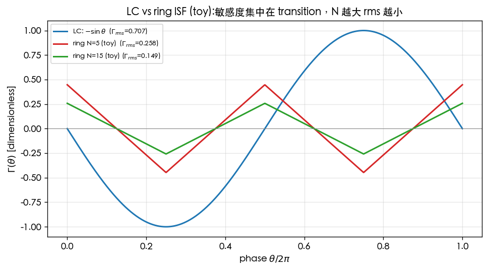
• Matching references: [P1] Fig. 7 (LC vs ring waveforms and ISFs); [P2] Fig. 8 ($\Gamma_{rms}$ vs $N$).
• How to read it: the LC ISF is a smooth single tone; the ring's energy is squeezed into narrow transitions — with more stages, each transition occupies a smaller fraction of the period, and $\Gamma_{rms}$ drops.
• Toy-model note: this site's gamma_triangular is a pedagogical toy ISF with "energy concentrated at the transitions", not a transistor-level extraction (see the isf_utils.py docstring).

The ring's $\Gamma_{rms}\propto N^{-3/2}$ scaling

[P2] quantifies the observation above into a scaling law ([P2] Eq.(16), p.794):

$$\Gamma_{rms}\propto N^{-3/2}$$

• Intuition: as the stage count $N$ increases, (i) each stage's transition becomes steeper and the ISF pulse narrower (rms drops), and (ii) the number of transitions per period grows but is diluted by the period length. Combined, this gives $\Gamma_{rms}^2\propto N^{-3}$ (i.e. $\Gamma_{rms}\propto N^{-3/2}$).

• Full expression: [P2] Eq.(16) is

  $$\Gamma_{rms}=\sqrt{\frac{2\pi^2}{3\eta^3}}\;\dfrac{1}{N^{1.5}},$$

  where $\eta$ is the stage-delay proportionality constant ([P2] Eq.(14), $\eta\approx1$ — not $\gamma$). The square root covers only the constant $2\pi^2/(3\eta^3)$; $1/N^{1.5}$ sits outside the radical, so $\Gamma_{rms}\propto N^{-3/2}$ (at $\eta=0.75$, this is $\approx4/N^{1.5}$, the solid line in [P2] Fig.8; [P2] Eq.(16), p.794 — re-verified in v7: the main text's statement "the $1/N^{1.5}$ dependence of $\Gamma_{rms}$", the $\eta=0.75$ numerical anchor, and an independent algebraic derivation from App.B Eq.(52)+(54) all agree on $N^{-3/2}$. A v3 audit misread the radical's scope and mistakenly changed this to $N^{-3/4}$, mislabeling it "verified" — that was a misreading, not a formula-vs-text inconsistency; v7 corrects it back).

• Key conclusion: [P2] further shows that under the constraint of fixed $f_0$ and power $P$, a single-ended ring's $1/f^2$ phase noise/jitter is nearly independent of the stage count $N$ ([P2] Sec.V, Eq.(23)/(25), p.796, $\mathcal{L}\big|_{1/f^2}\approx\dfrac{8}{3\eta}\,\dfrac{V_{DD}}{V_{char}}\,\dfrac{kT}{P}(\omega_0/\Delta\omega)^2$).

• Prefactor note: the prefactor of [P2] Eq.(23) is $\dfrac{8}{3\eta}$ ($\eta$ being the stage-delay proportionality constant of Eq.(14), $\approx1$); $\gamma$ enters only through $V_{char}=\Delta V/\gamma$. Its $V_T=0$ lower bound ([P2] Eq.(25)) is $\dfrac{16\gamma}{3\eta}$. (v2 mistakenly changed this to $8/(3\gamma)$ and mislabeled it "verified verbatim"; v3 corrected it against the original PDF, p.796.)

• Full LC-vs-ring discussion in lc_vs_ring; the random walk of accumulated jitter, $\sigma_{\Delta t}=\kappa\sqrt{\Delta t}$ ([P2] Eq.(8)), is in lab_03_ring_oscillator_toy_model.

Validity and failure conditions

Condition	When it holds	What happens when it fails
$\Gamma$ is a $2\pi$-periodic steady-state function	Parseval holds exactly	not usable when non-periodic (transient/injection)
white noise is flat (equal strength in every band)	$\sum c_n^2$ sums everything in one shot	colored noise must be weighted band by band — $\Gamma_{rms}$ alone is not enough
numerical-integration window aligned to one period	coefficients and Parseval reconcile	window missing the endpoint $2\pi$ → off-by-one; Parseval fails to reconcile
stationary noise	use $\Gamma_{rms}$ directly	cyclostationary noise requires $\Gamma_{eff}$ instead (see effective_isf)

Worked examples

These three problems follow the spec's Section 10.4 format: problem → step-by-step substitution (with units) → result → dimension check → one-line Python verification.

Worked example 1: $\Gamma_{rms}=1/\sqrt2$ for $\Gamma=-\sin$

Problem: for the ideal LC, $\Gamma(\theta)=-\sin\theta$. Find $\Gamma_{rms}$.

Step-by-step substitution: apply the definition directly, $\Gamma_{rms}^2=\dfrac{1}{2\pi}\displaystyle\int_0^{2\pi}\Gamma^2\,d\theta$.

$$\begin{aligned} \Gamma_{rms}^2 &=\frac{1}{2\pi}\int_0^{2\pi}(-\sin\theta)^2\,d\theta =\frac{1}{2\pi}\int_0^{2\pi}\sin^2\theta\,d\theta\\ &=\frac{1}{2\pi}\int_0^{2\pi}\frac{1-\cos2\theta}{2}\,d\theta =\frac{1}{2\pi}\left[\frac{\theta}{2}-\frac{\sin2\theta}{4}\right]_0^{2\pi} =\frac{1}{2\pi}\cdot\frac{2\pi}{2}=\frac12. \end{aligned}$$

Result: $\Gamma_{rms}=\sqrt{1/2}=\dfrac{1}{\sqrt2}\approx0.707$. The second line uses the half-angle identity $\sin^2\theta=\tfrac12(1-\cos2\theta)$; $\cos2\theta$ integrates to 0 over a full period.

Dimension check: $\Gamma=-\sin\theta$ is dimensionless → $\Gamma^2$ dimensionless → integrating over $\theta$ (rad), dividing by $2\pi$ (rad), and taking the square root leaves it dimensionless ✓.

import numpy as np
from simulations.common.isf_utils import gamma_lc_ideal, gamma_rms
theta = np.linspace(0.0, 2*np.pi, 4096, endpoint=True)   # include endpoint 2*pi
print(gamma_rms(theta, gamma_lc_ideal(theta)))            # -> 0.7071  (= 1/sqrt(2))

Worked example 2: $\Gamma_{rms}$ of the triangular (ring-toy) ISF

Problem: the ring's pedagogical toy ISF uses this site's gamma_triangular ($N=5$): a triangle wave with peak $P=1/\sqrt N=1/\sqrt5$, ramping linearly back and forth between $[-P,P]$ (two transitions per period). Find $\Gamma_{rms}$. (Toy model, not transistor-level.)

Step-by-step substitution: the triangle wave is linear on each basic ramp, so the mean square follows the standard result "mean square of a linear segment over $[-P,P]$ $=P^2/3$". Reason: write the linear segment as $\Gamma=P\,s$ (with $s$ sweeping uniformly from $-1$ to $1$),

$$\langle\Gamma^2\rangle=\frac{1}{2}\int_{-1}^{1}(P s)^2\,ds=\frac{P^2}{2}\cdot\frac{s^3}{3}\Big|_{-1}^{1}=\frac{P^2}{2}\cdot\frac{2}{3}=\frac{P^2}{3}.$$

Substituting $P=1/\sqrt5$:

$$\Gamma_{rms}^2=\frac{P^2}{3}=\frac{1/5}{3}=\frac{1}{15}\approx0.0667 \ \Rightarrow\ \Gamma_{rms}=\frac{1}{\sqrt{15}}\approx0.258.$$

Result: $\Gamma_{rms}\approx0.258$, far below the LC's 0.707 — consistent with the physics that "the ring squeezes its sensitivity into narrow transitions, the energy is flattened out, and $\Gamma_{rms}$ shrinks with $N$" (echoing the $\Gamma_{rms}\propto N^{-3/2}$ trend; the toy's $N$ dependence here is $1/\sqrt N$, not the real scaling).

Dimension check: $P$ is dimensionless (the ISF is dimensionless) → $\Gamma_{rms}$ dimensionless ✓.

import numpy as np
from simulations.common.isf_utils import gamma_triangular, gamma_rms
theta = np.linspace(0.0, 2*np.pi, 200001, endpoint=True)
print(gamma_rms(theta, gamma_triangular(theta, n_stages=5)))  # -> 0.2582  (= 1/sqrt(15))

Worked example 3: numerically verifying $\sum c_n^2=2\Gamma_{rms}^2$ (Parseval reconciliation)

Problem: for the triangular ISF of worked example 2 ($N=5$), compute $\sum_{n=0}^{\infty}c_n^2$ from the coefficient side and $2\Gamma_{rms}^2$ from the integral side, and verify that the two are equal.

Step-by-step substitution: from worked example 2, $2\Gamma_{rms}^2=2\times\dfrac{1}{15}=\dfrac{2}{15}\approx0.1333$. On the coefficient side, add up the squared $c_n$, remembering the half weight $c_0^2/2$ for $n=0$ (the triangle wave is symmetric, $c_0=0$, so DC contributes nothing). Parseval guarantees the two numbers are equal.

Result: $\sum_{n=0}^{\infty}c_n^2=2\Gamma_{rms}^2\approx0.1333$ ✓.

Dimension check: $c_n$ and $\Gamma_{rms}$ are all dimensionless; both sides agree ✓.

import numpy as np
from simulations.common.isf_utils import (
    gamma_triangular, compute_fourier_coefficients, gamma_rms,
)
theta = np.linspace(0.0, 2*np.pi, 4096, endpoint=True)
gamma = gamma_triangular(theta, n_stages=5)
a0, a, b, c, ph = compute_fourier_coefficients(theta, gamma, n_harmonics=32)
lhs = 0.5*c[0]**2 + np.sum(c[1:]**2)   # half weight for n=0
rhs = 2.0*gamma_rms(theta, gamma)**2
print(lhs, rhs)                        # -> ~0.1333 , 0.1333  (more harmonics, closer match)

• Feel: a triangle wave carries "infinitely many odd harmonics", so the coefficient side needs enough n_harmonics (e.g. 32) to approach $2\Gamma_{rms}^2$; taking too few harmonics (e.g. 8) slightly undershoots the integral value — which is itself a numerical portrait of "the ring ISF's energy spread across high harmonics".
• Full script: simulations/lab_05_fourier_isf.py; library: simulations/common/isf_utils.py.

Key takeaways

• Parseval: $\sum_{n=0}^{\infty}c_n^2=\dfrac{1}{\pi}\int_0^{2\pi}|\Gamma|^2dx=2\Gamma_{rms}^2$ ([P1] Eq.(20), p.185).
• $\Gamma_{rms}$ collapses the "band-by-band fold-back" into one shape metric; together with $q_{max}$ it sets the $1/f^2$ phase noise: $\mathcal{L}\propto\Gamma_{rms}^2/q_{max}^2$ ([P1] Eq.(21)).
• DC-factor convention: $c_0$ is the coefficient; the DC value is $c_0/2$; the $n=0$ term in the Parseval sum contributes $c_0^2/2$ (not $c_0^2$). Just copy the spec's equations.
• Ideal LC: $\Gamma_{rms}=1/\sqrt2\approx0.707$; canonical Example B with $\Gamma_{rms}=0.5$ gives $\mathcal{L}(1\text{MHz})\approx-148$ dBc/Hz.
• Ring: $\Gamma_{rms}\propto N^{-3/2}$ ([P2] Eq.(16), p.794; the radical covers only the constant, $\approx4/N^{1.5}$ at $\eta=0.75$, corroborated three ways by the main text and App.B; a v3 misreading of the radical's scope had this as $N^{-3/4}$, corrected back in v7).

Further reading

• Fourier coefficients of the ISF (the previous step): fourier_series_of_isf
• Using $\Gamma_{rms}$ to compute $1/f^2$ (the next step): white_noise_to_phase_noise
• LC-vs-ring design trade-offs: lc_vs_ring
• Cyclostationary correction: effective_isf
• Numerical-feel quick reference: numerical_feeling