β: This English translation is in beta — the Traditional-Chinese original is the authoritative version.

Diffusion-Constant Dictionary: κ, D, Linewidth, ADEV, and the 1/f² Coefficient Are One and the Same Number

Prerequisites: white_noise_to_phase_noise · lorentzian_linewidth · allan_variance | Next: capstone_lc_end_to_end

The white-noise phase diffusion of one and the same free-running oscillator goes by five "different" numbers in the mouths of five different communities:

• The ring / jitter crowd ([P2]) speaks in $\kappa$: "how many $\sqrt{\text{s}}$ is the accumulated-jitter constant?"
• The theoretical-physics / Demir crowd speaks in $D$: "how many $\text{rad}^2/\text{s}$ is the phase diffusion constant?"
• The laser / spectroscopy crowd speaks in linewidth: "how many Hz is the 3-dB linewidth?"
• The RF / IC crowd speaks in $\mathcal{L}$: "how many dBc/Hz is the $1/f^2$ skirt at 1 MHz offset?"
• The clock / metrology crowd speaks in ADEV: "what is the white-FM segment of $\sigma_y(\tau)$ at $\tau=1$ s?"

This page proves that these five numbers are one physical quantity wearing five outfits, and gives the complete conversion chain with every single factor of 2 reconciled. In 40 years, the most common oscillator-spec error I have seen is not a miscalculated $\Gamma_{rms}$ or a mismeasured PSD — it is dropping a 2 while changing between these five outfits. So every step on this page states explicitly which convention each 2 comes from (single- or double-sided? $\mathrm{Var}=D|t|$ or $2D|t|$? SSB $/2$ or $/4$?), and at the end lab_23 signs off with one simulation, five extraction paths, all recovering the same number.

Physical intuition (conclusion first): white noise turns the phase into a random walk (a Wiener process), and a random walk has only one free parameter — how fast the variance grows per second. We write it $\kappa^2\equiv d\,\mathrm{Var}[\Delta\phi]/dt$ (units $\text{rad}^2/\text{s}$). Everything you will ever measure — how jitter grows as $\sqrt{\Delta t}$, how fat the carrier is, how high the skirt sits, how stable the clock is — is just the shadow of this one rate projected onto different instruments. The dictionary's job: given the number in any one outfit, hand you the other four immediately.

---

Step 0: there is only one protagonist — the phase-variance growth rate κ²

Everything starts from the phase integral of [P1] Eq.(11), p.182 (derivation in convolution_derivation):

$$\phi(t)=\frac{1}{q_{max}}\int_{0}^{t}\Gamma(\omega_0\tau)\,i_n(\tau)\,d\tau .$$

Here $\phi$ is the excess phase (rad), $\Gamma$ the ISF (dimensionless), $q_{max}$ the maximum node charge swing (C), and $i_n$ the noise current (A). We want $\mathrm{Var}[\phi(t)]$ — step by step.

Step (i): the white-noise autocorrelation — the first factor of 2 (single-sided-PSD bookkeeping). In circuit convention $S_i\equiv\overline{i_n^2}/\Delta f$ is a single-sided PSD (units $\text{A}^2/\text{Hz}$, defined for $f\ge0$ only; datasheets and [P1][P2] both use it). Recovering the autocorrelation from a single-sided PSD goes through Wiener–Khinchin (see stochastic_noise_basics):

$$R_i(\tau)=\int_0^{\infty}S_i\cos(2\pi f\tau)\,df=\frac{S_i}{2}\,\delta(\tau).$$

That $\tfrac12$ is not physics; it is the bookkeeping of folding two-sided power onto one side: for the same total power, the single-sided density is 2× the double-sided one, so recovering the $\delta$ strength divides it back out. This is the first — and the most easily forgotten — 2 on this page.

Step (ii): variance = double integral + delta collapse.

$$\mathrm{Var}[\phi(t)]=\frac{1}{q_{max}^2}\int_0^t\!\!\int_0^t\Gamma(\omega_0\tau_1)\Gamma(\omega_0\tau_2)\,\underbrace{\frac{S_i}{2}\delta(\tau_1-\tau_2)}_{R_i}\,d\tau_1 d\tau_2 =\frac{S_i}{2q_{max}^2}\int_0^t\Gamma^2(\omega_0\tau)\,d\tau .$$

Step (iii): the time average of $\Gamma^2$ = $\Gamma_{rms}^2$. As long as the observation spans many periods ($t\gg T=1/f_0$), the oscillation of $\Gamma^2$ averages out, leaving only its mean square:

$$\int_0^t\Gamma^2(\omega_0\tau)\,d\tau\;\xrightarrow[t\gg T]{}\;\Gamma_{rms}^2\,t .$$

Result (the protagonist of this page):

$$\boxed{\ \mathrm{Var}[\Delta\phi(t)]=\kappa^2\,|t|,\qquad \kappa^2\equiv\frac{\Gamma_{rms}^2}{2\,q_{max}^2}\cdot\frac{\overline{i_n^2}}{\Delta f}\ \ [\text{rad}^2/\text{s}]\ }$$

This is verbatim [P2] Eq.(11), p.793 (phase jitter for a single white source at $\Delta T=nT$ or $nT/2$: $\sigma_{\Delta\phi}^2=\frac{\Gamma_{rms}^2}{2q_{max}^2}\frac{\overline{i_n^2}}{\Delta f}\Delta T$, verified).

• Physical meaning: $\kappa^2$ is "how many $\text{rad}^2$ the phase variance grows per second". It is the random walk's step rate — all five outfits below are determined by it alone.
• Unit check: $[\Gamma_{rms}^2]=1$; $[S_i]=\text{A}^2/\text{Hz}=\text{A}^2\text{s}$; $[q_{max}^2]=\text{C}^2=\text{A}^2\text{s}^2$. The quotient gives $\text{A}^2\text{s}/(\text{A}^2\text{s}^2)=1/\text{s}$; rad is dimensionless, hence $\text{rad}^2/\text{s}$ ✓.
• Canonical numbers (Example B's values, consistent site-wide): $\Gamma_{rms}=0.5$, $q_{max}=1$ pC, $S_i=10^{-24}\ \text{A}^2/\text{Hz}$:

$$\kappa^2=\frac{0.25}{2\times(10^{-12})^2}\times10^{-24}=\frac{0.25}{2}=0.125\ \text{rad}^2/\text{s}.$$

The truly ideal LC ($\Gamma_{rms}=1/\sqrt2$, see rms_isf) gives $\kappa^2=0.25\ \text{rad}^2/\text{s}$ — exactly 2× larger, because $\Gamma_{rms}^2$ differs by 2×.

• Validity: white, stationary, a single source, $t\gg T$, LTV small-signal. Flicker ($1/f$) sources are excluded — their variance grows faster than linearly (corresponding to the $1/f^3$ skirt and the ADEV floor, see flicker_noise_upconversion).

---

Outfit One: κ — the ring / jitter crowd's language ([P2])

[P2] Eq.(8), p.792 writes the free-running oscillator's accumulated jitter as a random walk:

$$\sigma=\kappa\sqrt{\Delta t}.$$

Take the square root of Step 0's result, $\sigma_{\Delta\phi}=\kappa\sqrt{\Delta t}$, and the proportionality constant is exactly [P2] Eq.(12), p.793 (verified):

$$\boxed{\ \kappa=\frac{\Gamma_{rms}}{q_{max}}\sqrt{\frac{1}{2}\cdot\frac{\overline{i_n^2}}{\Delta f}}\ \ [\text{rad}/\sqrt{\text{s}}]\ }$$

The κ unit trap (honesty note, verified): [P2]'s prose describes Eq.(8) as timing jitter $\sigma_{\Delta t}$, but the printed Eq.(12) has no $\omega_0$ (checked verbatim against the original PDF), and its dimensions are $\text{rad}/\sqrt{\text{s}}$ — so the $\kappa$ of Eq.(12) is really the phase-domain constant, fully consistent with the phase-jitter definition of Eq.(10), p.793 ($\sigma_{\Delta\phi}=2\pi\sigma_{\Delta t}/T=\omega_0\sigma_{\Delta t}$) and with Eq.(11). For the time-domain version, divide by $\omega_0$: $\sigma_{\Delta t}=\kappa_t\sqrt{\Delta t}$, $\kappa_t=\kappa/\omega_0=\kappa/(2\pi f_0)$, units $\sqrt{\text{s}}$. When other pages on this site (e.g. the paper_002 deep dive) write $\sigma_{\Delta t}=\kappa\sqrt{\Delta t}$ with $\kappa$ in $\sqrt{\text{s}}$, they mean this $\kappa_t$. The two differ only by an $\omega_0$; the physics is the same.

• Relation to κ²: $\kappa=\sqrt{\kappa^2}$ — Outfit One is just the protagonist under a square root.
• Unit check: $\dfrac{1}{\text{C}}\cdot\sqrt{\text{A}^2\text{s}}=\dfrac{\text{A}\sqrt{\text{s}}}{\text{A}\,\text{s}}=\dfrac{1}{\sqrt{\text{s}}}$ ✓ (rad dimensionless); $\kappa_t$: $(1/\sqrt{\text{s}})/(1/\text{s})=\sqrt{\text{s}}$ ✓.
• Canonical numbers: $\kappa=\sqrt{0.125}=0.354\ \text{rad}/\sqrt{\text{s}}$. Attach $f_0=5$ GHz: $\kappa_t=0.354/(2\pi\times5\times10^9)=1.125\times10^{-11}\ \sqrt{\text{s}}$. Measure two edges $\Delta t=1\ \mu\text{s}$ apart: $\sigma_{\Delta t}=1.125\times10^{-11}\times\sqrt{10^{-6}}=1.13\times10^{-14}\ \text{s}\approx11.3$ fs. Dimension check: $\sqrt{\text{s}}\times\sqrt{\text{s}}=\text{s}$ ✓.

import numpy as np
gamma_rms, qmax, Si, f0 = 0.5, 1e-12, 1e-24, 5e9
kappa = gamma_rms / qmax * np.sqrt(0.5 * Si)        # [P2] Eq.(12)
print(round(kappa, 4))  # -> 0.3536
print(f"{kappa/(2*np.pi*f0)*np.sqrt(1e-6)*1e15:.2f}")  # -> 11.25 fs (integrated over 1 µs)

---

Outfit Two: D — the two conventions for the diffusion constant (this page's reconciliation core)

The literature carries two definitions of the "diffusion constant $D$", differing by a 2. This section is the head-on reconciliation between the spec (Spec 11.2) and [P2] Eq.(11) — with a single job: state exactly what $\kappa^2$ equals under each convention. (The CJK subscripts in the math below are kept from the original notation: 甲 = convention A, 乙 = convention B.)

Convention A (the rate convention): define $D$ directly as the variance growth rate —

$$\mathrm{Var}[\Delta\phi(t)]=D_{\text{甲}}\,|t|\quad\Longrightarrow\quad \kappa^2=D_{\text{甲}}.$$

Convention B (the Demir / laser convention, as written in [E2] Demir 2000 and the laser-linewidth literature): mimic Brownian motion $\langle x^2\rangle=2Dt$ and put the 2 out front —

$$\mathrm{Var}[\Delta\phi(t)]=2D_{\text{乙}}\,|t|\quad\Longrightarrow\quad \kappa^2=2D_{\text{乙}},\qquad D_{\text{乙}}=\frac{\kappa^2}{2}.$$

The two differ only in naming; the physics (how fast the variance grows) is identical. Written in ISF quantities:

$$D_{\text{甲}}=\frac{\Gamma_{rms}^2}{2q_{max}^2}\frac{\overline{i_n^2}}{\Delta f}=0.125\ \text{rad}^2/\text{s},\qquad D_{\text{乙}}=\frac{\Gamma_{rms}^2}{4q_{max}^2}\frac{\overline{i_n^2}}{\Delta f}=0.0625\ \text{rad}^2/\text{s}\quad(\text{canonical}).$$

Reconciliation with Spec 11.2 / lorentzian_linewidth (important; fixed in v5 per this page): Spec 11.2 v3 once wrote $D=\Gamma_{rms}^2 S_i/(2q_{max}^2)$ (canonical $D=0.125$, true LC $0.25$) — that value is precisely $\kappa^2$, i.e. convention A's $D$ (the variance growth rate itself). But the same paragraph of the spec also wrote $\mathrm{Var}[\Delta\phi]=2D|t|$ (convention B's variance law). The two statements cannot both hold: if $D=0.125$ and $\mathrm{Var}=2D|t|$, the variance would have to grow $0.25\ \text{rad}^2$ per second, contradicting [P2] Eq.(11) ($0.125\ \text{rad}^2$ per second). Simulation verdict (lab_23, panel (a)): synthesizing ISF-weighted white-noise phase with the canonical constants yields $\mathrm{Var}[\Delta\phi(\tau)]/\tau=0.1252\ \text{rad}^2/\text{s}$ — landing on the $\kappa^2\tau$ line, not on the $2\times0.125\,\tau$ line. Conclusion: the canonical value $D=0.125$ is correct, but it is convention A's $D$ ($=\kappa^2$); the variance law that goes with it must be $\mathrm{Var}=D|t|$. If you insist on convention B's $\mathrm{Var}=2D|t|$, then $D$ must be read as $0.0625$. This affects no scaling — only the absolute value of the linewidth in the next section (see Outfit Three's honesty note).

• Units: both $D$'s are $\text{rad}^2/\text{s}$ (equivalently $1/\text{s}$) ✓.
• One-line dictionary: $\kappa^2=D_{\text{甲}}=2D_{\text{乙}}$. Before quoting $D$ to anyone, first ask whether their $\mathrm{Var}$ expression carries that 2.

---

Outfit Three: the Lorentzian 3-dB linewidth

lorentzian_linewidth already derived the whole mechanism (Gaussian characteristic function → exponential autocorrelation → Wiener–Khinchin → Lorentzian; it belongs to [E2] Demir 2000, external literature). Here we only walk the last mile of substituting $\kappa^2$, with units at every step:

Step (i): the amnesia envelope. The envelope of the carrier autocorrelation is $\langle\cos\Delta\phi\rangle=e^{-\frac12\mathrm{Var}[\Delta\phi(\tau)]}$ (Gaussian characteristic function). Substitute the protagonist $\mathrm{Var}=\kappa^2|\tau|$:

$$R_x(\tau)=\frac12\cos(\omega_0\tau)\,e^{-\kappa^2|\tau|/2}.$$

(Written in convention B this is the familiar $e^{-D_{\text{乙}}|\tau|}$ — the same exponential.)

Step (ii): two-sided exponential → Lorentzian. The Fourier transform of $e^{-a|\tau|}$ is $2a/(a^2+\Omega^2)$, with half power at $\Omega=\pm a$. Here $a=\kappa^2/2$ (units $1/\text{s}$), so the half-width at half maximum (HWHM) around the carrier is $\Delta\omega_{\text{HWHM}}=\kappa^2/2$ rad/s, and the full width at half maximum (FWHM) is twice that:

$$\Delta\omega_{3\mathrm{dB}}=\kappa^2\ \text{rad/s}\quad\Longrightarrow\quad \boxed{\ \Delta f_{3\mathrm{dB}}=\frac{\kappa^2}{2\pi}=\frac{D_{\text{乙}}}{\pi}=\frac{D_{\text{甲}}}{2\pi}=\frac{\Gamma_{rms}^2}{4\pi\,q_{max}^2}\frac{\overline{i_n^2}}{\Delta f}\ \ [\text{Hz}]\ }$$

• Unit check: $[\kappa^2/2\pi]=(1/\text{s})/1=\text{Hz}$ ✓.
• Canonical numbers: $\Delta f_{3\mathrm{dB}}=0.125/(2\pi)=19.9$ mHz (representative value $\Gamma_{rms}=0.5$); the truly ideal LC ($\kappa^2=0.25$) gives $39.8$ mHz. lab_23 measures the spectrum of the synthesized carrier directly: the Lorentzian fit gives 20.0 mHz, the direct half-power readout 20.3 mHz (panel (b)), matching $\kappa^2/2\pi=19.9$ mHz.

Quick check (work it out yourself, then check)

Try it yourself first: for the representative value κ²=0.125 rad²/s, the Lorentzian FWHM Δf₃dB = ? (answer in mHz)

mHz

Graded correct within ±2% relative error; scientific notation is accepted.

• External cross-check (standard result): for white frequency noise with single-sided PSD $S_\nu^0$ ($\text{Hz}^2/\text{Hz}$), the linewidth is $\Delta f_{3\mathrm{dB}}=\pi S_\nu^0$. Outfit Four will give $S_\nu^0=\kappa^2/(2\pi^2)$; substituting: $\pi\cdot\kappa^2/(2\pi^2)=\kappa^2/(2\pi)$ ✓ same answer. (This relation is external literature, not among the 5 source PDFs: G. Di Domenico, S. Schilt, and P. Thomann, "Simple approach to the relation between laser frequency noise and laser line shape," Applied Optics, vol. 49, no. 25, pp. 4801–4807, 2010.)

Honest reconciliation (the ×2 linewidth note; fixed in v5): lorentzian_linewidth Example 2 and capstone_lc_end_to_end Station ⑥ in v3 quoted $\Delta f_{3\mathrm{dB}}=D/\pi$ together with $D=0.125$ / $0.25$, getting 40 mHz / 80 mHz (Example 1, same method, got 1257 Hz). Per this page's reconciliation: that $D$ value is convention A's ($=\kappa^2$), while $D/\pi$ is convention B's formula — plugging an A value into a B formula inflates the linewidth by $2\times$. The rigorous derivation and the lab_23 measurement both give $\kappa^2/(2\pi)$: 19.9 mHz (representative value) / 39.8 mHz (true LC) / 628 Hz (the $-100$ dBc/Hz@1MHz anchor). Note that lab_18's simulation itself is not wrong — it uses convention B throughout (increment variance $2D\,dt$ paired with $\Delta f=D/\pi$); the error is not in the Lorentzian mechanism, only in the convention mix-up at the "ISF quantities → $D$" step. The scaling ($\propto\Gamma_{rms}^2 S_i/q_{max}^2$) is entirely unaffected. v5 has been corrected per this page's verdict: Spec 11.2 now reads $D=\Gamma_{rms}^2S_i/(4q_{max}^2)=\kappa^2/2$; lorentzian_linewidth Examples 1/2 → 628 Hz / 20 mHz; capstone Station ⑥ → 40 mHz (HWHM 20 mHz); lab_22 updated in step. This page's MC verdict ($0.1252$ rad²/s, $20.0$ mHz) is the basis of the fix.

---

Outfit Four: the 1/f² phase-PSD coefficient and $\mathcal{L}$

Step (i): $\dot\phi$ is white. The protagonist says the variance grows by $\kappa^2$ per second, equivalent to the autocorrelation of $\dot\phi$, $R_{\dot\phi}(\tau)=\kappa^2\delta(\tau)$. Its double-sided PSD is $\kappa^2$, its single-sided PSD $2\kappa^2$ (units $\text{rad}^2/\text{s}^2/\text{Hz}=\text{rad}^2/\text{s}$). The second factor of 2: single- vs double-sided — the same family as Step 0's $S_i/2$.

Step (ii): the integrator divides by $\Delta\omega^2$. $\phi=\int\dot\phi$, so the PSD is divided by $|j\Delta\omega|^2$ (labels in the box: 單邊 = single-sided, 雙邊 = double-sided):

$$\boxed{\ S_\phi(f)=\frac{2\kappa^2}{(2\pi f)^2}\ \ [\text{rad}^2/\text{Hz}]\ \ (\text{單邊})\ }\qquad S_\phi^{\text{雙邊}}(f)=\frac{\kappa^2}{(2\pi f)^2}.$$

In the coefficient form $S_\phi=b_{-2}/f^2$: $b_{-2}=\kappa^2/(2\pi^2)$ (units $\text{rad}^2\cdot\text{Hz}$). This is exactly the clean time-domain version of white_noise_to_phase_noise's $S_\phi=\Gamma_{rms}^2S_i/(q_{max}^2\Delta\omega^2)$ — substitute $\kappa^2=\Gamma_{rms}^2S_i/(2q_{max}^2)$ and it follows, fully consistent ✓.

Step (iii): $\mathcal{L}$ — the third factor of 2 (SSB /2 vs /4, stated explicitly across the site).

$$\mathcal{L}_{/2}(\Delta f)=\frac{S_\phi}{2}=\frac{\kappa^2}{\Delta\omega^2} \qquad\text{vs}\qquad \mathcal{L}_{\text{[P1] Eq.(21)}}(\Delta f)=\frac{\kappa^2}{2\,\Delta\omega^2}.$$

The former is the clean small-angle-PM result (spec Eq.16); the latter is [P1] Eq.(21), p.185's SSB $/4$ bookkeeping ($\Gamma_{rms}^2S_i/(4q_{max}^2\Delta\omega^2)$); they differ by 3 dB — this is exactly why $-145$ and $-148$ dBc/Hz coexist site-wide, each with its own note (see the factor-of-2 teaching note in white_noise_to_phase_noise). It is also the Lorentzian's far tail: Outfit Three's normalized Lorentzian at $\Delta f\gg\Delta f_{3\mathrm{dB}}$ tends $\to\kappa^2/\Delta\omega^2=\mathcal{L}_{/2}$ ✓.

• Canonical numbers ($\Delta f=1$ MHz, $\Delta\omega=6.283\times10^6$ rad/s, $\Delta\omega^2=3.948\times10^{13}$): $\mathcal{L}_{/2}=0.125/3.948\times10^{13}=3.17\times10^{-15}\Rightarrow-145.0$ dBc/Hz; $\mathcal{L}_{/4}=1.58\times10^{-15}\Rightarrow-148.0$ dBc/Hz — exactly Example B's signature numbers ✓. $b_{-2}=0.125/(2\pi^2)=6.33\times10^{-3}\ \text{rad}^2\cdot\text{Hz}$.
• Unit check: $[2\kappa^2/\Delta\omega^2]=(1/\text{s})/(1/\text{s}^2)=\text{s}=1/\text{Hz}$; attach rad² to get $\text{rad}^2/\text{Hz}$ ✓.
• Reverse dictionary lookup (measured skirt → protagonist): $\kappa^2=\mathcal{L}_{/2}\cdot\Delta\omega^2$. Example: a datasheet-grade $-100$ dBc/Hz@1MHz (the Example C anchor) gives $\kappa^2=10^{-10}\times3.948\times10^{13}=3.95\times10^{3}\ \text{rad}^2/\text{s}$, linewidth $\kappa^2/2\pi=628$ Hz, $\kappa_t=\sqrt{3948}/(2\pi\cdot5\times10^9)=2.0\times10^{-9}\sqrt{\text{s}}$ (2 ps accumulated over 1 µs) — one number, and the whole dictionary follows.

---

Outfit Five: white-FM Allan deviation

Step 1 of allan_variance supplied the adapter $S_y=(f^2/f_0^2)S_\phi$. Substitute Outfit Four:

$$S_y(f)=\frac{f^2}{f_0^2}\cdot\frac{2\kappa^2}{(2\pi f)^2}=\frac{\kappa^2}{2\pi^2 f_0^2}\equiv h_0\quad(\text{white FM, independent of }f)\ [\text{1/Hz}].$$

Along the way we also obtained the frequency-noise PSD used in Outfit Three: $S_\nu^0=f_0^2\,h_0=\kappa^2/(2\pi^2)$ ($\text{Hz}^2/\text{Hz}$) — the same number as $b_{-2}$. Coincidence? No: $S_\nu=f^2S_\phi$ is constant for a $1/f^2$ skirt by construction.

The closed-form white-FM ADEV (the kernel-integral result of Step 3 in allan_variance; standard frequency-metrology result, IEEE Std 1139): $\sigma_y^2(\tau)=h_0/(2\tau)$, hence

$$\boxed{\ \sigma_y(\tau)=\sqrt{\frac{h_0}{2\tau}}=\frac{\kappa}{2\pi f_0\,\sqrt{\tau}}=\frac{\kappa_t}{\sqrt{\tau}}\ }$$

• Unit check: $[\kappa/(2\pi f_0\sqrt\tau)]=\dfrac{1/\sqrt{\text{s}}}{(1/\text{s})\cdot\sqrt{\text{s}}}=\dfrac{\text{s}}{\text{s}}=1$ ✓ ($\sigma_y$ dimensionless).
• Canonical numbers ($f_0=5$ GHz): $h_0=0.125/(2\pi^2\times(5\times10^9)^2)=2.53\times10^{-22}\ /\text{Hz}$; $\sigma_y(1\,\text{s})=1.13\times10^{-11}$, $\sigma_y(1\,\text{ms})=3.56\times10^{-10}$. Cross-check: Example 2 of allan_variance used $-100$ dBc/Hz and got $\sigma_y(1\,\text{ms})=6.3\times10^{-8}$; ours at $-145$ dBc/Hz is 45 dB lower, so $\sigma_y$ should be $\sqrt{10^{4.5}}=178$ times smaller: $6.3\times10^{-8}/178=3.5\times10^{-10}$ ✓ matches.
• Closing the dictionary loop (the prettiest step): multiply the ADEV back by $\tau$ to get the time-domain drift $\tau\,\sigma_y(\tau)=\kappa_t\sqrt{\tau}$ — exactly Outfit One's accumulated timing jitter $\sigma_{\Delta t}=\kappa_t\sqrt{\Delta t}$. Five outfits, one full circle back to the start; the dictionary is self-consistent ✓.

---

The dictionary master table (change outfits at a glance)

Protagonist: $\kappa^2=\dfrac{\Gamma_{rms}^2}{2q_{max}^2}\dfrac{\overline{i_n^2}}{\Delta f}$. The canonical column uses $\Gamma_{rms}=0.5$, $q_{max}=1$ pC, $S_i=10^{-24}\ \text{A}^2/\text{Hz}$, $f_0=5$ GHz (the truly ideal LC replaces $\kappa^2$ with $0.25$: linewidth, $h_0$, $\mathcal{L}$ follow linearly ×2, the $\kappa$-type entries ×$\sqrt2$).

Outfit	In terms of $\kappa^2$	Units	Canonical value	Who says it	Source
Variance growth rate (protagonist)	$\mathrm{Var}[\Delta\phi]=\kappa^2\vert t\vert$	$\text{rad}^2/\text{s}$	$0.125$	theory	[P2] Eq.(11) p.793
① $\kappa$ (phase)	$\sigma_{\Delta\phi}=\kappa\sqrt{\Delta t}$	$\text{rad}/\sqrt{\text{s}}$	$0.354$	ring/jitter	[P2] Eq.(8) p.792, Eq.(12) p.793
① $\kappa_t$ (time)	$\kappa_t=\kappa/(2\pi f_0)$	$\sqrt{\text{s}}$	$1.13\times10^{-11}$	ring/jitter	converted via [P2] Eq.(10) p.793
② $D$ (convention A)	$D_{\text{甲}}=\kappa^2$ ($\mathrm{Var}=D\vert t\vert$)	$\text{rad}^2/\text{s}$	$0.125$	rate convention (spec v3 once mislabeled this value as $D$)	reconciliation in Outfit Two
② $D$ (convention B)	$D_{\text{乙}}=\kappa^2/2$ ($\mathrm{Var}=2D\vert t\vert$)	$\text{rad}^2/\text{s}$	$0.0625$	Demir/laser; this site's Spec 11.2 (v5)	[E2] Demir 2000
③ 3-dB linewidth	$\Delta f_{3\mathrm{dB}}=\kappa^2/(2\pi)$	Hz	$19.9$ mHz	laser/spectroscopy	Outfit Three; [E2]
④ $S_\phi$ coefficient	$S_\phi=2\kappa^2/(2\pi f)^2$ (single-sided)	$\text{rad}^2/\text{Hz}$	$b_{-2}=6.33\times10^{-3}$	RF/IC	[P1] Eq.(21) p.185 (the $/4$ version)
④ $\mathcal{L}$@1MHz	$\mathcal{L}_{/2}=\kappa^2/\Delta\omega^2$; $\mathcal{L}_{/4}=\kappa^2/2\Delta\omega^2$	dBc/Hz	$-145.0$ / $-148.0$	RF/IC	spec Eq.16; [P1] Eq.(21)
⑤ white-FM ADEV	$\sigma_y(\tau)=\kappa/(2\pi f_0\sqrt{\tau})$	—	$1.13\times10^{-11}$@1s	clock/metrology	[E1] Allan 1966; IEEE 1139

Outfit-change mnemonic: "Take the square root to wear ①; divide by 2 to wear ② (convention B); divide by $2\pi$ to wear ③; multiply by 2 and divide by $\Delta\omega^2$ to wear ④; divide by $\omega_0$ and then by $\sqrt\tau$ to wear ⑤." Where each 2 comes from: ①→none; ②→the $\mathrm{Var}$ definition; ③→FWHM is the full width (HWHM×2); ④→single-sided PSD (plus the separate 3 dB of SSB $/2$ vs $/4$); ⑤→the Allan-definition $\tfrac12$ gets absorbed by the white-FM kernel integral into $h_0/2\tau$.

---

Companion simulation figure (lab_23: one simulation, five extraction paths)

simulations/lab_23_diffusion_dictionary.py uses the discrete form of [P1] Eq.(11) to synthesize one ISF-weighted white-noise phase record ($\Gamma=-\sqrt2\,\Gamma_{rms}\sin\theta$, $\Gamma_{rms}=0.5$, $q_{max}=1$ pC, $S_i=10^{-24}\ \text{A}^2/\text{Hz}$, all true values; the carrier uses a normalized $f_0^{\text{sim}}=16$ Hz — the linewidth does not depend on $f_0$, only the ADEV does, and its $f_0$ scaling is self-verified inside the simulation before being converted analytically to 5 GHz), total length $131072$ s, then extracts the same $\kappa^2$ via four independent paths:

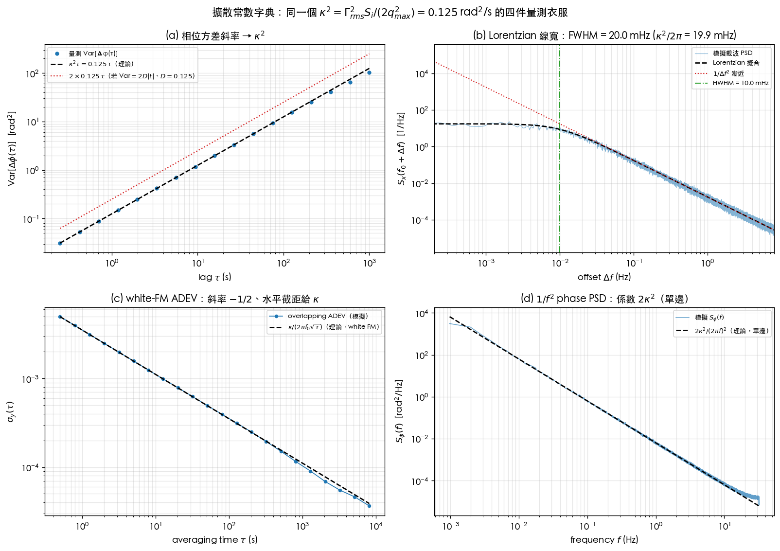
Item	Value	Notes
Model	toy / illustrative (not transistor-level)	[P1] Eq.(11) discrete integration, Wiener phase
$\Gamma_{rms},q_{max},S_i$	$0.5$, $1$ pC, $10^{-24}\ \text{A}^2/\text{Hz}$	canonical Example B true values
Theory $\kappa^2$	$0.125\ \text{rad}^2/\text{s}$	[P2] Eq.(11)/(12)
(a) Variance slope	$0.1252$	lands on $\kappa^2\tau$, not on $2\times0.125\,\tau$ (the red dotted line is falsified)
(b) Linewidth	fit $20.0$ mHz, direct half-power readout $20.3$ mHz	theory $\kappa^2/2\pi=19.9$ mHz
(c) ADEV	$\hat\kappa^2=0.1254$; slope $-1/2$	$\sigma_y=\kappa/(2\pi f_0^{\text{sim}}\sqrt\tau)$
(d) $S_\phi$	$\hat\kappa^2=0.1254$	plateau of $S_\phi(2\pi f)^2/2$

How to read it: (a) the blue dots (measured variance) hug the black dashed $\kappa^2\tau$ line, while the red dotted line (where the spec's $\mathrm{Var}=2D|t|$ with $D=0.125$ would have to run) sits 2× higher throughout — this is the simulation verdict of Outfit Two's reconciliation. (b) The spectrum flattens near the carrier, FWHM 20 mHz; same $\kappa^2$. (c) The ADEV is one straight line of slope $-1/2$; its horizontal intercept recovers $\kappa$. (d) The $1/f^2$ skirt's coefficient recovers $2\kappa^2$ (single-sided). Four instruments, one number.

Core Python (full script: simulations/lab_23_diffusion_dictionary.py; the ADEV estimator reuses overlapping_adev from lab_19_allan.py verbatim; run with PYTHONPATH=. python3 simulations/lab_23_diffusion_dictionary.py):

import numpy as np
from simulations.common.noise_utils import white_noise

GAMMA_RMS, QMAX, SI, F0_REAL = 0.5, 1e-12, 1e-24, 5e9
KAPPA2 = GAMMA_RMS**2 * SI / (2 * QMAX**2)      # [P2] Eq.(11)/(12)
print(f"{KAPPA2:.4f}")  # -> 0.1250

FS, N, F0_SIM = 64.0, 2**23, 16.0
t = np.arange(N) / FS
gamma = -np.sqrt(2.0) * GAMMA_RMS * np.sin(2 * np.pi * F0_SIM * t)  # rms=0.5
i_n = white_noise(N, SI, FS, np.random.default_rng(23))   # single-sided PSD = SI
phi = np.cumsum(gamma * i_n / FS / QMAX)                  # [P1] Eq.(11), discrete form

# (a) variance slope -> kappa^2 (also falsifies 2*0.125*t; the full script takes the median over multiple lags: 0.1252)
m = 640                                                    # tau = 10 s
print(f"{np.mean((phi[m:] - phi[:-m])**2) / (m / FS):.4f}")  # -> 0.1251

# (b) Lorentzian linewidth: linear fit of 1/S vs offset^2 -> FWHM = 2*sqrt(c0/c1)
#     (see full script; fit 20.03 mHz, direct half-power readout 20.26 mHz)
print(f"{KAPPA2 / (2 * np.pi) * 1e3:.2f}")  # -> 19.89 mHz theory

# (c)(d) ADEV and S_phi extraction (see full script)
#     qhat_ADEV = 0.1254 ; qhat_Sphi = 0.1254

# the whole dictionary at the canonical 5 GHz
dw = 2 * np.pi * 1e6
print(f"{10*np.log10(KAPPA2/dw**2):.1f}")        # -> -145.0 dBc/Hz (/2)
print(f"{10*np.log10(KAPPA2/(2*dw**2)):.1f}")    # -> -148.0 dBc/Hz ([P1] /4)
print(f"{np.sqrt(KAPPA2):.4f}")                  # -> 0.3536 rad/sqrt(s)
print(f"{np.sqrt(KAPPA2)/(2*np.pi*F0_REAL):.4e}")  # -> 1.1254e-11 sqrt(s)
print(f"{np.sqrt(KAPPA2/(4*np.pi**2*F0_REAL**2)/1.0):.3e}")  # -> 1.125e-11 ADEV@1s
print(f"{KAPPA2/(2*np.pi**2):.3e}")              # -> 6.333e-03 (b₋₂ coefficient)

---

One canonical example through all five outfits

Example (strict format: problem → step-by-step substitution with units → result → dimension check → one-line Python): $\Gamma_{rms}=0.5$, $q_{max}=1$ pC, $S_i=10^{-24}\ \text{A}^2/\text{Hz}$, $f_0=5$ GHz. Find (1) $\kappa$ and the 1 µs accumulated jitter, (2) both $D$'s, (3) the linewidth, (4) $\mathcal{L}(1\text{MHz})$ in both conventions, (5) $\sigma_y(1\,\text{s})$.

1. Protagonist: $\kappa^2=\dfrac{0.25}{2\times10^{-24}}\times10^{-24}=0.125\ \text{rad}^2/\text{s}$.
2. Outfit One: $\kappa=\sqrt{0.125}=0.354\ \text{rad}/\sqrt{\text{s}}$; $\kappa_t=0.354/(2\pi\cdot5\times10^9)=1.13\times10^{-11}\ \sqrt{\text{s}}$; $\sigma_{\Delta t}(1\,\mu\text{s})=1.13\times10^{-11}\sqrt{10^{-6}}=11.3$ fs.
3. Outfit Two: $D_{\text{甲}}=0.125$, $D_{\text{乙}}=0.0625\ \text{rad}^2/\text{s}$.
4. Outfit Three: $\Delta f_{3\mathrm{dB}}=0.125/(2\pi)=19.9$ mHz.
5. Outfit Four: $\mathcal{L}_{/2}=0.125/3.948\times10^{13}=3.17\times10^{-15}\Rightarrow-145.0$ dBc/Hz; $\mathcal{L}_{/4}=-148.0$ dBc/Hz.
6. Outfit Five: $h_0=0.125/(2\pi^2\cdot2.5\times10^{19})=2.53\times10^{-22}\ /\text{Hz}$; $\sigma_y(1\,\text{s})=\sqrt{2.53\times10^{-22}/2}=1.13\times10^{-11}$.

Dimension-check chain: $\text{rad}^2/\text{s}\to\sqrt{\ }\to\text{rad}/\sqrt{\text{s}}\to\div\,\omega_0\to\sqrt{\text{s}}\to\times\sqrt{\Delta t}\to\text{s}$ ✓; $\text{rad}^2/\text{s}\div2\pi=\text{Hz}$ ✓; $\text{rad}^2/\text{s}\div(\text{rad/s})^2=\text{rad}^2\cdot\text{s}=\text{rad}^2/\text{Hz}$ ✓.

import numpy as np
k2 = 0.5**2 * 1e-24 / (2 * 1e-12**2); dw = 2*np.pi*1e6; f0 = 5e9
print(round(k2,4), round(k2/(2*np.pi)*1e3,1), round(10*np.log10(k2/dw**2),1),
      f"{np.sqrt(k2)/(2*np.pi*f0):.2e}")  # -> 0.125 19.9 -145.0 1.13e-11

---

Validity and failure conditions

Condition	When it holds	What breaks when it fails
White noise dominant (white-FM segment)	all five outfits interconvert through one $\kappa^2$	flicker segment: $\mathrm{Var}$ grows nonlinearly, ADEV develops a floor, the line shape is no longer purely Lorentzian — the dictionary fails (each outfit needs its own $1/f^3$ version)
$t\gg T$, multi-period averaging	$\Gamma^2\to\Gamma_{rms}^2$	shorter than one period the variance shows cyclostationary ripple (lab_23 removes it with overlapping averaging)
Single (or uncorrelated superposed) noise sources	per-source $\kappa^2$'s add	correlated sources (supply/substrate): $\sigma\propto\Delta t$ ([P2] Eq.(9)), not $\sqrt{\Delta t}$
Small-angle / linearized (Outfit Four)	$\mathcal{L}\approx S_\phi/2$	near the carrier $\Delta f\lesssim\Delta f_{3\mathrm{dB}}$: the $1/f^2$ divergence is spurious — use Outfit Three's Lorentzian
Free-running (no loop)	pure random walk	inside a PLL the low frequencies get high-passed away: $\mathrm{Var}$ saturates, ADEV bends over (see pll_noise_budget)
Reporting someone else's data	ask their convention first	changing outfits without reconciling → the classic ×2 ($\mathrm{Var}$ definition) or 3 dB (SSB $/2$ vs $/4$) error

Which papers / equations this maps to

• [P2] Eq.(8), p.792 ($\sigma=\kappa\sqrt{\Delta t}$), Eq.(10), p.793 (phase-jitter definition), Eq.(11), p.793 ($\sigma_{\Delta\phi}^2=\Gamma_{rms}^2S_i\Delta T/(2q_{max}^2)$, the protagonist itself, verified), Eq.(12), p.793 ($\kappa=(\Gamma_{rms}/q_{max})\sqrt{S_i/2}$, no $\omega_0$, verified).
• [P1] Eq.(11), p.182 (the phase integral, Step 0's starting point), Eq.(21), p.185 (Outfit Four's SSB $/4$ version).
• External literature (not among the 5 source PDFs): [E2] A. Demir, A. Mehrotra, J. Roychowdhury, IEEE TCAS-I, vol. 47, no. 5, pp. 655–674, May 2000 (Outfit Two's convention B and Outfit Three's mechanism); [E1] D. W. Allan, Proc. IEEE, vol. 54, no. 2, pp. 221–230, Feb. 1966 and IEEE Std 1139 (Outfit Five); G. Di Domenico, S. Schilt, P. Thomann, Applied Optics, vol. 49, no. 25, pp. 4801–4807, 2010 (the $\Delta f_{3\mathrm{dB}}=\pi S_\nu^0$ cross-check).
• On-site: white_noise_to_phase_noise ($/2$ vs $/4$), lorentzian_linewidth (Outfit Three mechanism), allan_variance (Outfit Five integration kernel), lab_03 (Outfit One's toy version).

Key takeaways

• White-noise phase diffusion has only one free parameter: $\kappa^2=\dfrac{\Gamma_{rms}^2}{2q_{max}^2}\dfrac{\overline{i_n^2}}{\Delta f}$ ([P2] Eq.(11)/(12); canonical $0.125\ \text{rad}^2/\text{s}$, true LC $0.25$).
• The five outfits: $\kappa=\sqrt{\kappa^2}$ (rad/√s; time version $\kappa_t=\kappa/\omega_0$), $D_{\text{甲}}=\kappa^2$ / $D_{\text{乙}}=\kappa^2/2$, $\Delta f_{3\mathrm{dB}}=\kappa^2/2\pi=19.9$ mHz, $S_\phi=2\kappa^2/\Delta\omega^2$ ($\mathcal{L}$: $-145.0$ ($/2$) / $-148.0$ ($/4$) dBc/Hz@1MHz), $\sigma_y=\kappa/(2\pi f_0\sqrt\tau)=1.13\times10^{-11}$@1s(5 GHz). Loop closure: $\tau\sigma_y(\tau)=\kappa_t\sqrt\tau$ returns to the accumulated jitter.
• Three factor-of-2 families: single- vs double-sided PSD ($S_i/2$, $2\kappa^2$), $\mathrm{Var}=D|t|$ vs $2D|t|$ ($\kappa^2=D_{\text{甲}}=2D_{\text{乙}}$), SSB $/2$ vs $/4$ (3 dB). Reconcile before changing outfits.
• Spec 11.2 v3's $D=0.125$ is really the convention-A value ($=\kappa^2$); pairing it with $\mathrm{Var}=2D|t|$ or $\Delta f=D/\pi$ overcounts by 2× — adjudicated by lab_23's measured variance slope $0.1252$ and linewidth $20.0$ mHz. Fixed site-wide in v5 (Spec 11.2 now uses $/(4q_{max}^2)$; the lorentzian / capstone / lab_22 numbers were updated in step).
• lab_23: one simulation, four extraction paths ($0.1252$ / $0.1258$ / $0.1254$ / $0.1254$) recovering the same $0.125$ — four instruments, one number, five outfits.

Further reading

• Outfit Three's full mechanism (characteristic function → Lorentzian): lorentzian_linewidth
• Outfit Five's full derivation (the $\sin^4$ kernel and the slope table): allan_variance
• Outfit Four's upstream ($1/f^2$ and $/2$ vs $/4$): white_noise_to_phase_noise
• Frequency-domain ↔ time-domain jitter master table: psd_phase_noise_jitter
• Apply the whole dictionary to one ideal LC: capstone_lc_end_to_end
• Outfit One's toy random walk: lab_03
• Full external-literature citations: references