Lorentzian Linewidth: Resolving the 1/f² Divergence Paradox at Δf→0

β: This English translation is in beta — the Traditional-Chinese original is the authoritative version.

Prerequisites: white_noise_to_phase_noise (the signature $1/f^2$ result [P1] Eq.(21)), rms_isf ($\Gamma_{rms}^2/q_{max}^2$ sets the phase diffusion), stochastic_noise_basics (autocorrelation ↔ Wiener–Khinchin).

The previous page white_noise_to_phase_noise derived the signature result of oscillator phase noise, [P1] Eq.(21): the phase-noise skirt caused by white noise is

$$\mathcal{L}\{\Delta\omega\}=10\log_{10}\!\left(\frac{\Gamma_{rms}^2}{q_{max}^2}\cdot\frac{\overline{i_n^2}/\Delta f}{4\,\Delta\omega^2}\right).$$

The equation is beautiful, but it hides a disturbing mathematical pathology: the denominator contains $\Delta\omega^2$, so as the offset $\Delta\omega\to0$ (infinitely close to the carrier), the bracket $\to\infty$ and $\mathcal{L}\to+\infty$. Read literally, the noise power density at the exact center of the carrier is infinite — which is obviously wrong: a real oscillator has finite total power (namely its output power) and cannot pack infinite power density into any single frequency.

This page resolves that paradox head-on. Conclusion first: $1/\Delta\omega^2$ is the far-offset asymptote of the "phase linearization" approximation, not the truth near the carrier. Honestly account for the random-walk nature of the phase, and the carrier spectrum flattens near the carrier into a Lorentzian, with a finite peak, conserved total power, and a naturally defined finite 3-dB linewidth $\Delta f_{3\mathrm{dB}}=D/\pi$.

Physical intuition (conclusion first): white noise keeps kicking the phase, so $\phi(t)$ does not settle at any value; like a drunkard's walk it random-walks without bound (a Wiener process). The phase variance grows linearly: $\mathrm{Var}[\Delta\phi]=2D|t|$. The carrier $\cos(\omega_0t+\phi)$ therefore gradually loses memory: the longer the separation, the larger and less correlated the phase difference, so the autocorrelation $R_x(\tau)$ decays exponentially. The Fourier transform of an exponentially decaying autocorrelation is a Lorentzian — a bell-shaped line of finite height and finite width. $1/f^2$ is merely the tail of this Lorentzian "far from center." Near the center it must flatten, because "complete phase amnesia" can at most spread the power flat — it can never make it diverge.

This page follows the complete step-by-step Lorentzian derivation of spec 11.2 throughout. The mechanism used here — "phase diffusion → exponential autocorrelation → Lorentzian" — is external literature, corresponding mainly to [E2] A. Demir, A. Mehrotra, and J. Roychowdhury, "Phase Noise in Oscillators: A Unifying Theory and Numerical Methods for Characterization," IEEE Trans. Circuits Syst. I, vol. 47, no. 5, pp. 655–674, May 2000 (DOI: 10.1109/81.847872), not among the 5 source PDFs downloaded on this site (volume/issue/pages/DOI verified; see [E2] in references). [P1] itself obtains $1/f^2$ by linearization but never addresses the $\Delta\omega\to0$ divergence; the phase-diffusion model of Demir et al. is exactly the standard tool that fills that gap.

Step 0: The root of the problem — the phase is a random walk, not a fixed value

Return to the phase integral of [P1] Eq.(11) (see convolution_derivation):

$$\phi(t)=\frac{1}{q_{max}}\int_{-\infty}^{t}\Gamma(\omega_0\tau)\,i_n(\tau)\,d\tau .$$

The integral of white noise $i_n$ is a Wiener process — a Brownian-motion-style random walk. Its key property: no restoring force (the phase is the Floquet $\lambda_1=0$ neutral direction, see derivation_floquet_ppv), so the phase never returns to some equilibrium value; it diffuses without bound.

• Mathematical signature: the variance of integrated white noise grows linearly with time (this is the defining property of a Wiener process). Write the proportionality constant as $2D$:

$$\operatorname{Var}[\Delta\phi(t)]=\big\langle(\phi(t+t_0)-\phi(t_0))^2\big\rangle=2D\,|t|.$$

Here $D$ is called the phase diffusion constant, in units of $\text{rad}^2/\text{s}$ (spec 11.2). $|t|$ carries an absolute value because the variance is the same looking forward or backward (stationary increments).

• Unit check: $[\operatorname{Var}\Delta\phi]=\text{rad}^2$; right-hand side $[2D]\cdot[t]=(\text{rad}^2/\text{s})\cdot\text{s}=\text{rad}^2$ ✓.

• Why linear and not something else: white noise is uncorrelated across time; integrating $N$ independent increments makes the variances add linearly, like "summing $N$ dice rolls" ($N\propto t$) — this is the origin of the $\sqrt{t}$ walk and the $t$ variance, and it is exactly the same thing as $\sigma_{\Delta t}\propto\sqrt{\Delta t}$ in numerical_feeling (accumulated jitter is the time-domain version of the phase walk).

This step already exposes the seed of the paradox: the $1/f^2$ derivation treats $\phi$ as "small, linearizable, bounded"; but the real $\phi$ is an unbounded walk. When you ask "what happens infinitely close to the carrier ($\Delta\omega\to0$, i.e., observing infinitely long, $t\to\infty$)", $\phi$ has long since wandered to $\gg 1$ rad and the linearization has broken down. So the divergence is not physics — it is an approximation used where it fails.

Step 1: Carrier autocorrelation — turning the phase walk into exponential decay via the Gaussian characteristic function

Write the carrier as (the pure-phase version of [P1] Eq.(1); amplitude $A$ held constant, phase only):

$$x(t)=A\cos\big(\omega_0 t+\phi(t)\big).$$

We want its autocorrelation function (the average product of the signal with itself delayed by $\tau$):

$$R_x(\tau)=\big\langle x(t)\,x(t+\tau)\big\rangle .$$

Step (i): expand the two cosines with the product-to-sum identity. Let $\Delta\phi\equiv\phi(t+\tau)-\phi(t)$:

$$x(t)x(t+\tau)=A^2\cos(\omega_0t+\phi(t))\cos(\omega_0(t+\tau)+\phi(t+\tau)).$$

Using $\cos\alpha\cos\beta=\tfrac12[\cos(\alpha-\beta)+\cos(\alpha+\beta)]$:

$$x(t)x(t+\tau)=\frac{A^2}{2}\Big[\cos\big(\omega_0\tau+\Delta\phi\big)+\cos\big(2\omega_0t+\omega_0\tau+\phi(t)+\phi(t+\tau)\big)\Big].$$

• The slow term $\cos(\omega_0\tau+\Delta\phi)$ is independent of absolute time $t$ (it contains only $\tau$ and the phase difference) and survives the averaging.
• The fast term contains $2\omega_0t$; time-averaging over $t$ (or averaging over the random phase) kills it — it oscillates near $2\omega_0$ and is invisible to any long-term carrier average. Drop it.

Hence

$$R_x(\tau)=\frac{A^2}{2}\big\langle\cos(\omega_0\tau+\Delta\phi)\big\rangle.$$

Step (ii): move the average inside using the Gaussian characteristic function. Expand $\cos(\omega_0\tau+\Delta\phi)= \cos\omega_0\tau\cos\Delta\phi-\sin\omega_0\tau\sin\Delta\phi$. $\Delta\phi$ is zero-mean Gaussian (integrated white noise → Gaussian; and the distribution is symmetric, so $\langle\sin\Delta\phi\rangle=0$):

$$R_x(\tau)=\frac{A^2}{2}\Big[\cos\omega_0\tau\,\langle\cos\Delta\phi\rangle-\sin\omega_0\tau\,\underbrace{\langle\sin\Delta\phi\rangle}_{=0}\Big]=\frac{A^2}{2}\cos\omega_0\tau\,\langle\cos\Delta\phi\rangle.$$

The remaining $\langle\cos\Delta\phi\rangle$ uses the Gaussian characteristic function — for a zero-mean Gaussian variable $\Delta\phi\sim\mathcal{N}(0,\sigma^2)$,

$$\big\langle e^{j\Delta\phi}\big\rangle=e^{-\sigma^2/2}\quad\Longrightarrow\quad\langle\cos\Delta\phi\rangle=\operatorname{Re}\big\langle e^{j\Delta\phi}\big\rangle=e^{-\sigma^2/2}.$$

This is the mathematical pivot of this page: for a Gaussian, "the average of a complex exponential" equals "$e^{-\tfrac12\text{variance}}$". Substitute Step 0's $\sigma^2=\operatorname{Var}[\Delta\phi(\tau)]=2D|\tau|$:

$$\langle\cos\Delta\phi\rangle=e^{-\tfrac12\cdot 2D|\tau|}=e^{-D|\tau|}.$$

Step (iii): combine to get the carrier autocorrelation (spec 11.2). Absorb $A^2$ into the normalization (adopting the unit-power convention $A^2/2\to\tfrac12$, consistent with lab_18):

$$\boxed{\ R_x(\tau)=\frac{1}{2}\cos(\omega_0\tau)\,e^{-D|\tau|}\ }$$

• Physical meaning: $\cos(\omega_0\tau)$ is the carrier's own oscillation; $e^{-D|\tau|}$ is the memory-loss envelope — the longer the separation, the more phase difference accumulates and the smaller $\langle\cos\Delta\phi\rangle$ gets: the autocorrelation decays exponentially. Larger $D$ (fiercer noise) means faster memory loss.
• Unit check: $[D|\tau|]=(\text{rad}^2/\text{s})\cdot\text{s}=\text{rad}^2$? — note that $D|\tau|$ appears in an exponent and must be dimensionless. The convention here treats the "$\text{rad}^2$" of $D$ as dimensionless (phase is dimensionless radians to begin with), so $D$ is effectively $[1/\text{s}]$ and $D|\tau|$ is dimensionless ✓. $R_x$ is dimensionless (power-normalized) ✓.
• Connection to [P1]: [P1] never wrote this $e^{-D|\tau|}$; it stops at "phase small, linear." Once you admit the phase is an unbounded walk, this exponential decay is the only self-consistent outcome (the core of [E2] Demir 2000).

Step 2: Wiener-Khinchin — exponentially decaying autocorrelation ⇒ Lorentzian spectrum

Wiener-Khinchin theorem: the power spectral density $S_x(\omega)$ of a stationary random process is the Fourier transform of its autocorrelation $R_x(\tau)$:

$$S_x(\omega)=\int_{-\infty}^{\infty}R_x(\tau)\,e^{-j\omega\tau}\,d\tau .$$

Substitute Step 1's $R_x(\tau)=\tfrac12\cos(\omega_0\tau)e^{-D|\tau|}$. Splitting $\cos(\omega_0\tau)= \tfrac12(e^{j\omega_0\tau}+e^{-j\omega_0\tau})$ gives two identical two-sided-exponential transforms, shifted to $\pm\omega_0$. We only need the branch around $+\omega_0$ (near the positive-frequency carrier).

The standard transform used (Fourier transform of the two-sided exponential — the canonical Lorentzian pair):

$$\int_{-\infty}^{\infty}e^{-D|\tau|}\,e^{-j\Omega\tau}\,d\tau=\frac{2D}{D^2+\Omega^2}.$$

Work it out by hand (split into the $\tau>0$ and $\tau<0$ halves):

$$\begin{aligned} \int_{-\infty}^{\infty}e^{-D|\tau|}e^{-j\Omega\tau}d\tau &=\int_{0}^{\infty}e^{-(D+j\Omega)\tau}d\tau+\int_{0}^{\infty}e^{-(D-j\Omega)\tau}d\tau\\ &=\frac{1}{D+j\Omega}+\frac{1}{D-j\Omega}=\frac{(D-j\Omega)+(D+j\Omega)}{D^2+\Omega^2}=\frac{2D}{D^2+\Omega^2}. \end{aligned}$$

Let the offset angular frequency near the carrier be $\Omega=\omega-\omega_0\equiv\Delta\omega$ (absorbing the $e^{j\omega_0\tau}$ branch of the $\cos$, which amounts to shifting the frequency origin to the carrier), and carry the $R_x$ prefactor $\tfrac12\cdot\tfrac12=\tfrac14$:

$$\boxed{\ S_x(\Delta\omega)\propto\frac{D}{D^2+\Delta\omega^2}\ }\qquad(\textbf{Lorentzian, spec 11.2}).$$

• This is the Lorentzian: a bell-shaped line centered on the carrier, with a finite peak, symmetric left and right.
• See how the divergence is gone: as $\Delta\omega\to0$, $S_x\to D/D^2=1/D$ — finite! The peak is $1/D$, not infinity. The divergence is cured.
• Unit/shape check: the two denominator terms $D^2+\Delta\omega^2$ share the same dimension (both $[\text{s}^{-2}]$), so the shape of the ratio is correct; the overall constant is fixed by total-power normalization (see Step 4).

Why the far offset returns to $1/f^2$ (consistent with [P1])

When $\Delta\omega\gg D$ (far enough from the carrier), the denominator $D^2+\Delta\omega^2\approx\Delta\omega^2$:

$$S_x(\Delta\omega)\xrightarrow[\Delta\omega\gg D]{}\frac{D}{\Delta\omega^2}\propto\frac{1}{\Delta\omega^2}.$$

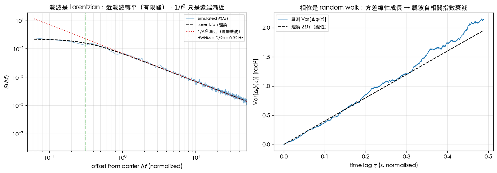
The far-offset asymptote is exactly $1/f^2$ — in full agreement with [P1] Eq.(21). So the Lorentzian does not overturn [P1]; it embeds [P1]'s $1/f^2$ into a complete lineshape that flattens near the carrier: $1/f^2$ far out, flat close in, with the corner at $\Delta\omega\approx D$. The figure below overlays all three (simulation / Lorentzian theory / $1/f^2$ asymptote).

Step 3: 3-dB linewidth (FWHM) = D/π

The Lorentzian's full width at half maximum (FWHM) is what engineers call the "3-dB linewidth" or simply the "linewidth." Find it: the peak at $\Delta\omega=0$ is $D/D^2=1/D$; at half maximum $S_x=\tfrac12\cdot\tfrac1D$:

$$\frac{D}{D^2+\Delta\omega^2}=\frac{1}{2D}\quad\Longrightarrow\quad D^2+\Delta\omega^2=2D^2\quad\Longrightarrow\quad\Delta\omega=\pm D.$$

So the half-maximum points sit at $\Delta\omega=\pm D$ (rad/s).

• HWHM (half width): $\Delta\omega_{\text{HWHM}}=D$ rad/s $\Rightarrow$ $\Delta f_{\text{HWHM}}=\dfrac{D}{2\pi}$ Hz.
• FWHM (3-dB full width): twice the HWHM, $\Delta\omega_{\text{FWHM}}=2D$ rad/s $\Rightarrow$

$$\boxed{\ \Delta f_{3\mathrm{dB}}=\frac{2D}{2\pi}=\frac{D}{\pi}\ \text{Hz}\ }\qquad(\textbf{spec 11.2}).$$

• Physical meaning: larger $D$ (fiercer noise, faster phase amnesia) means a wider linewidth and a "fatter" carrier. An ideal noiseless oscillator has $D\to0$ → linewidth $\to0$ → it degenerates into a delta line (pure carrier).
• Unit check: $[D/\pi]=(1/\text{s})/(\text{dimensionless})=\text{Hz}$ ✓.
• Where "3 dB" comes from: half height $=$ half power $=10\log_{10}(1/2)=-3.01$ dB, hence "3-dB linewidth."

Step 4: Total power conservation — the Lorentzian flattens the infinity into a finite integral

The most fatal consequence of the near-carrier $1/f^2$ divergence: integrating $1/\Delta\omega^2$ from $0$ diverges ($\int_0 d(\Delta\omega)/\Delta\omega^2=\infty$), which would say the phase-noise power is infinite. The Lorentzian cures this, because the Lorentzian's integral converges. Using the standard integral $\int_{-\infty}^{\infty}\dfrac{d\Omega}{D^2+\Omega^2}=\dfrac{\pi}{D}$:

$$\int_{-\infty}^{\infty}\frac{D}{D^2+\Delta\omega^2}\,d(\Delta\omega)=D\cdot\frac{\pi}{D}=\pi\quad(\text{finite}).$$

• Physical meaning: summing the power over all offsets gives a finite constant — exactly equal to the carrier's total power (after proper normalization). The phase walk merely smears the power originally concentrated in a delta line into a Lorentzian of finite width; no total power is lost (energy conservation). This is "total power conservation" (the key teaching point of spec 11.2).
• Compare with the delta line: as $D\to0$ the Lorentzian $\to\pi\,\delta(\Delta\omega)$ (infinitely tall and thin), degenerating back into the ideal carrier; for $D > 0$ it is flattened into a finite peak. The power never diverged — it was only redistributed.

The paradox resolved in one sentence: the $1/f^2$ divergence is a "false divergence" — it comes from forcing the unbounded phase walk into a bounded linear approximation. The real spectrum must flatten into a Lorentzian near the carrier (peak $=1/D$, width $=D/\pi$, total power $=$ carrier power, conserved). [P1] Eq.(21)'s $1/f^2$ holds only for $\Delta\omega\gg D$; it is the Lorentzian's far tail.

Step 5: Connecting to the ISF — expressing D in terms of Γrms and qmax

Now connect the abstract $D$ back to [P1]'s ISF quantities. Matching "the two expressions for the near-carrier $1/f^2$ skirt" pins down $D$.

From the Lorentzian side: far out, $S_x\to D/\Delta\omega^2$. Write it as a phase PSD — the double-sided phase PSD of a Wiener phase ($\mathrm{Var}=2D|t|$) is $2D/\Delta\omega^2$; this site keeps its books in single-sided PSD throughout (consistent with jitter_kernels), so

$$S_\phi(\Delta\omega)=\frac{4D}{\Delta\omega^2}\qquad[\text{rad}^2/\text{Hz}]\ (\text{single-sided}).$$

From the ISF side (the clean time-domain version from the previous page, $S_\phi=\Gamma_{rms}^2 S_i/(q_{max}^2\Delta\omega^2)$, writing $S_i=\overline{i_n^2}/\Delta f$):

$$S_\phi(\Delta\omega)=\frac{\Gamma_{rms}^2}{q_{max}^2}\cdot\frac{\overline{i_n^2}/\Delta f}{\Delta\omega^2}.$$

Set them equal (same $1/\Delta\omega^2$ skirt, so the coefficients must match):

$$4D=\frac{\Gamma_{rms}^2}{q_{max}^2}\cdot\frac{\overline{i_n^2}}{\Delta f}\quad\Longrightarrow\quad\boxed{\ D=\frac{\Gamma_{rms}^2}{4q_{max}^2}\cdot\frac{\overline{i_n^2}}{\Delta f}=\frac{\kappa^2}{2}\ }\qquad(\textbf{spec 11.2, v5 corrected}).$$

Substituting into Step 3's linewidth formula gives the 3-dB linewidth directly in ISF quantities:

$$\boxed{\ \Delta f_{3\mathrm{dB}}=\frac{D}{\pi}=\frac{\Gamma_{rms}^2}{4\pi\,q_{max}^2}\cdot\frac{\overline{i_n^2}}{\Delta f}=\frac{\kappa^2}{2\pi}\ }\qquad(\textbf{spec 11.2, v5 corrected}).$$

• Design message: linewidth $\propto\Gamma_{rms}^2/q_{max}^2\cdot S_i$ — the same set of knobs as [P1] Eq.(21)'s $\mathcal{L}$! For a narrow linewidth (a clean carrier), you still increase the charge swing $q_{max}$, suppress $\Gamma_{rms}$, and lower the noise PSD $S_i$. The Lorentzian introduces no new knob; it merely repackages the same physical quantities into "linewidth," a directly measurable number.
• Unit check: $[D]=\dfrac{1}{\text{C}^2}\cdot\dfrac{\text{A}^2}{\text{Hz}}=\dfrac{\text{A}^2}{\text{A}^2\text{s}^2}\cdot\text{s}=\dfrac{1}{\text{s}}$ (using $\text{C}=\text{A}\cdot\text{s}$ and $\text{Hz}^{-1}=\text{s}$) ✓, so $D/\pi$ is in Hz ✓.
• Factor-of-2 note (the clean version after the v5 correction): $D$ is a physical quantity (the decay rate of $R_x$, $\kappa^2/2$) and is independent of the bookkeeping convention for $\mathcal{L}$. Only $\mathcal{L}$ changes: the clean time-domain version is $\mathcal{L}=2D/\Delta\omega^2=\kappa^2/\Delta\omega^2$; [P1] Eq.(21)'s SSB $/4$ version is $\mathcal{L}=D/\Delta\omega^2$ — the famous 3 dB lives in $\mathcal{L}$, not in $D$. (v3 had mistakenly stuffed $\kappa^2$ into $D/\pi$ as if it were $D$, making the linewidth 2× too large; fixed in v5 — MC adjudication in diffusion_dictionary and lab_23.) This page is consistent with lab_18 throughout (lab_18 generates directly with $\mathrm{Var}=2D\,dt$, so the mechanism check is unaffected by the mapping).

Companion simulation figure

simulations/lab_18_lorentzian.py synthesizes a carrier $x=\cos(2\pi f_0t+\phi)$ from a segment of Wiener phase (accumulated white noise, $\phi=\operatorname{cumsum}(\text{N}(0,2D\,dt))$), estimates its spectrum with Welch, and overlays the Lorentzian theory and the $1/f^2$ asymptote; the right panel directly measures $\operatorname{Var}[\Delta\phi(\tau)]$ to verify its linear growth ($=2D\tau$).

Item	Value (lab_18)	Notes
Model	toy / illustrative (not transistor-level)	Wiener phase synthesized directly, labeled in normalized units
Carrier $f_0$	$400$ (normalized)	Arbitrary carrier; only the relative offset matters
Phase diffusion $D$	$2.0\ \text{rad}^2/\text{s}$	The single knob controlling the linewidth
Phase increment	$d\phi\sim\mathcal{N}(0,\,2D/f_s)$	Wiener: variance $=2D\,dt$
3-dB linewidth	$\Delta f_{3\mathrm{dB}}=D/\pi\approx0.64$ Hz	FWHM; HWHM $=D/2\pi\approx0.32$ Hz
Near carrier	Flattens into a finite peak $\propto1/D$	No longer diverges
Far from carrier	$\propto1/\Delta f^2$ asymptote	Consistent with [P1] Eq.(21)

How to read the left panel: at large offsets, the blue curve (simulated spectrum) slides down along the red dotted line ($1/\Delta f^2$ asymptote); approaching the carrier, the blue curve departs from $1/f^2$, hugs the black dashed line (Lorentzian), and flattens; the green dash-dot line marks the HWHM $=D/2\pi$ position — exactly where the corner happens. One glance at this figure says it all: $1/f^2$ is the tail; the Lorentzian is the whole picture. How to read the right panel: the measured $\operatorname{Var}[\Delta\phi(\tau)]$ (blue) lands precisely on the $2D\tau$ line (black dashed), confirming that the phase really is a linearly diffusing random walk — the very root of the exponential autocorrelation and hence the Lorentzian.

Interactive: same L(f_ref) spec, two lineshapes, smeared away by RBW

The figure above is the white-FM case; beyond_lorentzian proves that under flicker FM the same machinery yields a near-Gaussian line core instead of a Lorentzian, with linewidths that can differ by two orders of magnitude for the same spec point. The widget below overlays both lineshapes on the same axes and lets you sweep a spectrum analyzer's resolution bandwidth (RBW) — see for yourself how the "flattening" gets smeared away by the instrument's own resolution once the RBW is too wide:

Lineshape explorer: same L(f_ref) spec, two noise colors, RBW smearing

Dominant near-carrier noise:

L(10 kHz)-71.0 dBc/Hz

RBW (log)100 = 100 Hz

FWHM_true

49.9 Hz

apparent width @ this RBW

130 Hz

RBW

100 Hz

Model: a single spec point, L at 10 kHz (time-domain "/2" convention), is mapped to the near-carrier lineshape two ways. White FM(lorentzian_linewidth.md): unilateral S_phi = 4D / Delta-omega^2 fixes the phase diffusion constant D, giving an exact Lorentzian with FWHM = D/pi. Flicker FM(beyond_lorentzian.md Part A): b_-3 = S_phi times f_ref^3 fixes the 1/f^3 level; with a low-frequency cutoff f_l = 1/32 Hz (an observation-time artifact, not a device parameter — the page shows the dependence on f_l is only logarithmic), the frozen-log Gaussian-envelope approximation gives FWHM ≈ 2·sqrt(2 ln 2)·sqrt(b_-3 · L*) — an approximation the page itself quotes as roughly 2% off the exact numeric Fourier transform, not an exact result. Both curves are then convolved (direct 512-point discrete convolution, no FFT) with a Gaussian resolution-bandwidth kernel of FWHM = RBW to produce the "measured" trace. Toy/illustrative: real spectrum analyzers, cross-correlation instruments, and residual white-FM skirts (see beyond_lorentzian.md) all modify this picture further.

How to read it: fix a single spec point $\mathcal{L}(10\,\text{kHz})$ and toggle white FM / flicker FM to see how different FWHM_true is (tens-to-hundreds of Hz for white FM versus thousands of Hz for flicker FM — up to a hundredfold difference for the same number); then drag the RBW slider to the right and watch when the gray dashed curve (true lineshape) and the blue solid curve (RBW-convolved "measured" trace) part ways — once RBW is much larger than the linewidth, all you measure is a wide, featureless hump, and the flattening / near-Gaussian shoulder information is gone.

Core Python (full script: simulations/lab_18_lorentzian.py):

import numpy as np
from scipy.signal import welch

RNG = np.random.default_rng(18)
fs, n, f0, D = 4096.0, 2**20, 400.0, 2.0          # D = phase diffusion [rad^2/s]
t = np.arange(n) / fs

# Wiener phase: increments ~ N(0, 2 D dt) -> Var[phi(t)] = 2 D t
dphi = RNG.standard_normal(n) * np.sqrt(2 * D / fs)
phi = np.cumsum(dphi)
x = np.cos(2 * np.pi * f0 * t + phi)

f, P = welch(x, fs=fs, nperseg=2**16, scaling="density")   # spectrum: the carrier is a Lorentzian
off = f - f0
lor = D / (D**2 + (2 * np.pi * off)**2)                     # Lorentzian theory
fwhm = D / np.pi                                            # 3-dB linewidth = D/pi Hz

Worked examples

Both problems follow the strict format: problem → step-by-step substitution (with units) → result → dimension check → one-line Python verification. Example 1 works backward from a "real PN spec" to $D$ and the linewidth (the most design-flavored calculation); Example 2 works forward from the ISF quantities.

Example 1 (canonical: from 5 GHz, $-100$ dBc/Hz @ 1 MHz back to $D$ and the linewidth): a $f_0=5$ GHz oscillator measures $\mathcal{L}(1\,\text{MHz})=-100$ dBc/Hz with a $1/f^2$ slope. Find the phase diffusion $D$ and the 3-dB linewidth $\Delta f_{3\mathrm{dB}}$.

Step-by-step substitution:

1. Convert dBc/Hz back to linear. $\mathcal{L}=-100$ dBc/Hz means $\mathcal{L}_{\text{lin}}(1\,\text{MHz})=10^{-100/10}=10^{-10}\ /\text{Hz}$.

2. Get the phase PSD from $\mathcal{L}\approx\tfrac12 S_\phi$. $S_\phi(1\,\text{MHz})=2\mathcal{L}_{\text{lin}}=2\times10^{-10}\ \text{rad}^2/\text{Hz}$.

3. Extrapolate the coefficient using the $1/f^2$ shape. Single-sided $S_\phi(\Delta\omega)=\dfrac{4D}{\Delta\omega^2}$; at $\Delta f=1$ MHz: $\Delta\omega=2\pi\times10^6=6.283\times10^6$ rad/s, $\Delta\omega^2=3.948\times10^{13}$. Hence

$$4D=S_\phi\cdot\Delta\omega^2=2\times10^{-10}\times3.948\times10^{13}=7.896\times10^{3}\ \text{rad}^2/\text{s}.$$

4. Solve for $D$. $D=\dfrac{7.896\times10^3}{4}=1.974\times10^{3}\ \text{rad}^2/\text{s}$.

5. Compute the 3-dB linewidth. $\Delta f_{3\mathrm{dB}}=\dfrac{D}{\pi}=\dfrac{1.974\times10^3}{3.1416}\approx6.28\times10^{2}\ \text{Hz}\approx0.63\ \text{kHz}$.

Result: $D\approx1.97\times10^{3}\ \text{rad}^2/\text{s}$, 3-dB linewidth $\approx628$ Hz $\approx0.63$ kHz.

Intuition check: a 5 GHz oscillator at $-100$ dBc/Hz@1MHz actually has a carrier that is a Lorentzian about 0.63 kHz wide — a fractional linewidth of $1.26\times10^{-7}$ relative to the 5 GHz carrier (equivalent to a $Q$ on the order of $\sim 8\times10^6$). If the measurement resolution bandwidth (RBW) is far wider than 0.63 kHz, what you see is a "spike" smeared flat by the RBW, and the Lorentzian flattening is completely invisible; to see it you need $\sim100$ Hz-class RBW or cross-correlation methods. This is why everyday PN plots show only $1/f^2$ and never the Lorentzian plateau — the measurement resolution cannot get close enough to the carrier.

Dimension check: $[4D]=[S_\phi]\cdot[\Delta\omega^2]=\dfrac{\text{rad}^2}{\text{Hz}}\cdot\dfrac{\text{rad}^2}{\text{s}^2}$; with $\text{Hz}^{-1}=\text{s}$ and treating rad as dimensionless, $=\dfrac{1}{\text{s}}\cdot\text{s}\cdot\dfrac{1}{\text{s}^2}\cdot\text{s}=\dfrac{1}{\text{s}}$... which simplifies to $[D]=\text{rad}^2/\text{s}=1/\text{s}$, $[D/\pi]=\text{Hz}$ ✓.

import numpy as np
L_dbc = -100.0                      # dBc/Hz @ 1 MHz, 1/f^2 slope
df = 1e6
L_lin = 10**(L_dbc/10)             # = 1e-10 /Hz (intermediate value)
S_phi = 2 * L_lin                  # L ~ S_phi/2  -> rad^2/Hz
dw = 2*np.pi*df
D = S_phi * dw**2 / 4              # single-sided S_phi = 4D/dw^2  -> D
linewidth = D / np.pi             # 3-dB linewidth [Hz]
print(round(D), "rad^2/s ;", round(linewidth), "Hz")   # -> 1974 rad^2/s ; 628 Hz

Example 2 (forward from the ISF quantities to $D$ and the linewidth): use the numbers of the previous page's canonical Example B — $q_{max}=1$ pC, $\Gamma_{rms}=0.5$, $S_i=\overline{i_n^2}/\Delta f=10^{-24}\ \text{A}^2/\text{Hz}$. Find $D$ and the 3-dB linewidth.

Step-by-step substitution:

1. Compute $D=\dfrac{\Gamma_{rms}^2}{4q_{max}^2}\,S_i$. $\dfrac{\Gamma_{rms}^2}{4q_{max}^2}=\dfrac{0.25}{4\times(10^{-12})^2}=\dfrac{0.25}{4\times10^{-24}}=6.25\times10^{22}\ \text{C}^{-2}$.

2. Multiply by $S_i$: $D=6.25\times10^{22}\times10^{-24}=0.0625\ \text{rad}^2/\text{s}$.

3. Linewidth. $\Delta f_{3\mathrm{dB}}=\dfrac{D}{\pi}=\dfrac{0.0625}{3.1416}\approx0.0199\ \text{Hz}\approx20\ \text{mHz}$.

Result: $D=0.0625\ \text{rad}^2/\text{s}$, 3-dB linewidth $\approx20$ mHz.

Intuition cross-check: this "single ideal white-noise source" set of numbers corresponds to the previous page's clean time-domain version $\mathcal{L}(1\text{MHz})\approx-145$ dBc/Hz (the SSB $/4$ convention gives $-148$; this page uses the time-domain $/2$ version throughout, so $-145$ is the self-consistent baseline) — about 45 dB cleaner than Example 1's $-100$ dBc/Hz ($-100-(-145)=45$), so the linewidth is also much narrower (20 mHz vs 628 Hz, narrower by about $3\times10^4$×, $\approx 45$ dB as a power ratio, self-consistent ✓). This verifies that "linewidth and $\mathcal{L}$ are the same physics, only packaged differently": $\mathcal{L}$ lower by 45 dB $\Leftrightarrow$ $D$ and the linewidth smaller by about $10^{4.5}$×.

Alignment with the capstone's $40$ mHz ($\Gamma_{rms}^2$ packaging, not an error): this example uses the spec representative value $\Gamma_{rms}=0.5$ ($\Gamma_{rms}^2=0.25$), giving $D=0.0625\ \text{rad}^2/\text{s}$ and a linewidth $\approx20$ mHz; whereas the main ridge of capstone_lc_end_to_end uses the truly ideal LC value $\Gamma_{rms}=1/\sqrt2$ ($\Gamma_{rms}^2=0.5$, exactly twice), giving $D=0.125\ \text{rad}^2/\text{s}$ and a linewidth $\approx40$ mHz. Both numbers are correct — the $2\times$ difference is exactly the $\Gamma_{rms}^2$ packaging ($0.5$ vs $0.25$), not a mistake on either page (it matches the 3-dB gap of $-145$ vs $-148$ dBc/Hz at capstone station ⑤, $10\log_{10}2=3.01$ — the same thing). This page takes the representative value $0.5$ to align with the site-wide canonical Example B; the capstone consistently uses the ideal $-\sin$ value $1/\sqrt2$.

Dimension check: $[D]=\text{C}^{-2}\cdot\dfrac{\text{A}^2}{\text{Hz}}=\text{A}^{-2}\text{s}^{-2}\cdot\text{A}^2\text{s}=\dfrac{1}{\text{s}}$ ✓, $[D/\pi]=\text{Hz}$ ✓.

import numpy as np
gamma_rms, qmax, Si = 0.5, 1e-12, 1e-24
D = gamma_rms**2 / (4 * qmax**2) * Si      # rad^2/s (v5: 4q^2)
linewidth = D / np.pi                       # Hz
print(D, "rad^2/s ;", round(linewidth, 4), "Hz")   # -> 0.0625 rad^2/s ; 0.0199 Hz

(Both problems use the v5-corrected mapping $D=\Gamma_{rms}^2S_i/(4q_{max}^2)=\kappa^2/2$. $D$ and the linewidth are physical quantities, independent of the $\mathcal{L}$ bookkeeping convention; the SSB $/2$ vs $/4$ 3 dB affects only $\mathcal{L}$ — see the Step 5 note and diffusion_dictionary. Full library: simulations/common/noise_utils.py, simulations/lab_18_lorentzian.py.)

Validity and failure conditions

Condition	When it holds	What happens when it fails
Phase is a pure random walk (white noise dominant)	Autocorrelation $e^{-D\lvert\tau\rvert}$, spectrum purely Lorentzian	With flicker ($1/f^3$) the near-carrier lineshape is no longer a plain Lorentzian; the general Demir form is needed
Phase difference $\Delta\phi$ is Gaussian	Characteristic function $\langle\cos\Delta\phi\rangle=e^{-\sigma^2/2}$ is exact	Strong nonlinearity / large injection makes $\Delta\phi$ non-Gaussian and the approximation loses accuracy
Small $D$ (narrow linewidth, high $Q$)	Lorentzian and far-offset $1/f^2$ cleanly separated	Large $D$ (very noisy) broadens the whole line and the $1/f^2$ region shrinks
Stable amplitude (tracking phase only)	A single parameter $D$ suffices	With strong AM-PM the amplitude noise must be included as well
Measurement RBW $\ll D/\pi$	The Lorentzian plateau is measurable	Too-wide RBW shows only a $1/f^2$ spike; the flattening is invisible

Which papers / equations this corresponds to

• This page's mechanism (phase diffusion → exponential autocorrelation → Lorentzian → linewidth $D/\pi$) is external literature, not among the 5 source PDFs: [E2] Demir–Mehrotra–Roychowdhury 2000 (DOI 10.1109/81.847872, see references).
• The far-offset $1/f^2$ asymptote and the link $D=\Gamma_{rms}^2S_i/(4q_{max}^2)$ connect back to [P1] Eq.(21), p.185 (see white_noise_to_phase_noise).
• Root of the phase integral / random walk: [P1] Eq.(11), p.182 (see convolution_derivation and the $\lambda_1=0$ neutral direction in derivation_floquet_ppv).
• Accumulated jitter $\propto\sqrt{\Delta t}$ is the time-domain version of the same random walk ([P2] Eq.(8), p.792, see lab_03).

Key takeaways

• The $1/f^2$ divergence at $\Delta\omega\to0$ is a false divergence: it comes from forcing an unbounded phase random walk into a linear approximation.
• The phase is a Wiener process: $\operatorname{Var}[\Delta\phi]=2D|t|$ ($D$ = phase diffusion, $\text{rad}^2/\text{s}$).
• Gaussian characteristic function $\langle e^{j\Delta\phi}\rangle=e^{-\sigma^2/2}$ → carrier autocorrelation $R_x(\tau)=\tfrac12\cos(\omega_0\tau)e^{-D|\tau|}$.
• Wiener-Khinchin → Lorentzian $S\propto\dfrac{D}{D^2+\Delta\omega^2}$: flattens near the carrier (peak $=1/D$, no divergence), returns to $1/f^2$ far out, total power conserved (integral $=\pi$, finite).
• 3-dB linewidth $\Delta f_{3\mathrm{dB}}=\dfrac{D}{\pi}$ Hz; ISF link $D=\dfrac{\Gamma_{rms}^2}{4q_{max}^2}\dfrac{\overline{i_n^2}}{\Delta f}=\dfrac{\kappa^2}{2}$, so linewidth $=\dfrac{\Gamma_{rms}^2}{4\pi q_{max}^2}\dfrac{\overline{i_n^2}}{\Delta f}=\dfrac{\kappa^2}{2\pi}$ — the same knobs as $\mathcal{L}$ (v5-corrected mapping).
• Canonical: 5 GHz, $-100$ dBc/Hz@1MHz → $D\approx1.97\times10^3\ \text{rad}^2/\text{s}$, linewidth $\approx628$ Hz; representative-value ISF example → $D=0.0625$, linewidth $\approx20$ mHz (true LC: $D=0.125$, $\approx40$ mHz).
• The whole machinery is [E2] Demir 2000 external literature, not among the 5 source PDFs (DOI verified).

Further reading

• diffusion_dictionary (v5): κ↔D↔linewidth↔ADEV↔S_φ — the five outfits of the same quantity reconciled in one place (source of the MC adjudication for this page's D mapping).

• beyond_lorentzian (v5): when the white-noise assumption fails (1/f³) the lineshape is no longer Lorentzian; plus the non-stationarity viewpoint that "a free-running oscillator strictly has no S_φ."

• Upstream $1/f^2$ derivation (what this page corrects): white_noise_to_phase_noise

• Root of the phase integral (origin of the Wiener process): convolution_derivation

• $\lambda_1=0$ neutral direction (why the phase walks unboundedly): derivation_floquet_ppv

• The same walk in the time domain (accumulated jitter): lab_03

• Integrating $\mathcal{L}$ back into rms jitter: numerical_feeling

• Full citation of external literature [E2] Demir 2000: references