β: This English translation is in beta — the Traditional-Chinese original is the authoritative version.

Translator's note: all equations are preserved byte-for-byte from the original. Chinese labels appearing inside math read as follows: 單邊 = single-sided, 雙邊 = double-sided, 時域 = time-domain, 線寬 = linewidth, 噪 = noise strength, 無因次 = dimensionless, 甲 = convention "A".

Beyond the Lorentzian: 1/f³ Lineshape and Nonstationarity — What the Instrument Actually Measures

Prerequisites: lorentzian_linewidth (the full white-noise → Lorentzian chain and the "spurious divergence"), flicker_noise_upconversion (where the $1/f^3$ skirt comes from), stochastic_noise_basics (stationarity, Wiener–Khinchin) | Next: allan_variance (the canonical time-domain tool for characterizing flicker FM), measurement_and_spurs (instrumentation practicalities)

lorentzian_linewidth resolved the spurious divergence of $1/f^2$ as $\Delta\omega\to0$ with one clean logical chain: phase random walk ($\operatorname{Var}[\Delta\phi]=2D|t|$) → Gaussian characteristic function → exponential autocorrelation → Lorentzian lineshape. But the first link of that chain hides an assumption: the noise driving the phase is white. In a real oscillator, the skirt closest to the carrier is usually $1/f^3$ (flicker FM, see flicker_noise_upconversion) — so is the close-in lineshape still Lorentzian?

This page answers two questions:

1. Part A (lineshape): under flicker FM, $\operatorname{Var}[\Delta\phi(t)]$ no longer grows linearly but as $t^2\times\log$ (with an explicit role for a low-frequency cutoff $f_l$); the characteristic-function step therefore yields a near-Gaussian line core, not a Lorentzian.
2. Part B (nonstationarity): the free-running $\phi(t)$ is a random walk, so strictly speaking $S_\phi(f)$ does not exist (it is not a stationary process and has no stationary PSD); what the instrument really measures is the spectrum of $V(t)=\cos(\omega_0t+\phi)$ — which is stationary (the [E2] Demir view). Every $S_\phi$ formula on this site is a conditional spectrum under "finite observation time, offset $\gg$ linewidth"; the two descriptions agree exactly within that range.

Physical intuition (conclusion first): the lineshape is set by the "speed profile of phase memory loss". Under white noise the phase variance accumulates linearly ($\propto t$), the memory-loss envelope is the exponential $e^{-D|t|}$, and its Fourier transform is a Lorentzian. Under flicker FM, low-frequency noise parks the frequency itself on one side for long stretches, and the phase variance accumulates almost as $t^2$ (up to a log) — like a "walk with drift" — so the memory-loss envelope becomes the near-Gaussian $e^{-(\text{const})t^2\log}$, and the Fourier transform of a Gaussian is again a Gaussian: the line core becomes a bell-shaped Gaussian with shoulders far steeper than a Lorentzian's. For the very same $\mathcal{L}(10\,\text{kHz})$ spec, the white-noise version has a 50 Hz linewidth and the flicker version 3.1 kHz — a dBc/Hz number at one offset does not determine the linewidth at all; the noise "color" does. This is the main event of the lab_29 numerical demo.

Try it: the lorentzian_linewidth page embeds an interactive explorer — a slider for the same $\mathcal{L}(10\,\text{kHz})$ spec, a white FM / flicker FM toggle, and a spectrum-analyzer RBW slider — so you can see this page's "same spec, 100× difference in linewidth" conclusion first-hand, plus how too-wide an RBW smears away the flattening / near-Gaussian shoulder.

---

Part A: the $1/f^3$ lineshape of flicker FM

Step 0: the Lorentzian's hidden assumption, and single-/double-sided bookkeeping (factor-of-2 discipline)

The derivation chain of lorentzian_linewidth is:

$$\operatorname{Var}[\Delta\phi(t)]=2D|t| \;\Rightarrow\; \langle\cos\Delta\phi\rangle=e^{-\operatorname{Var}/2}=e^{-D|\tau|} \;\Rightarrow\; S_x(\Delta\omega)\propto\frac{D}{D^2+\Delta\omega^2},\quad \Delta f_{3\mathrm{dB}}=\frac{D}{\pi}.$$

The first link — variance grows linearly — holds only for white frequency noise (white FM: the PSD of $\dot\phi$ is flat). This page swaps that link for flicker FM and watches how the whole chain changes.

First, nail down the bookkeeping (this site's factor-of-2 discipline). Let the single-sided PSD of $\dot\phi$ for white FM be $W_0$ (units $\text{rad}^2/\text{s}^2/\text{Hz}=\text{rad}^2/\text{s}$). Step 1 will prove rigorously that $\operatorname{Var}[\Delta\phi(t)]=\tfrac{W_0}{2}|t|$, so $\operatorname{Var}=2D|t|$ corresponds to $W_0=4D$, and the phase spectrum (integrator $1/\Delta\omega^2$) is:

$$S_\phi^{\text{單邊}}(f)=\frac{4D}{(2\pi f)^2},\qquad S_\phi^{\text{雙邊}}(f)=\frac{2D}{(2\pi f)^2},\qquad \mathcal{L}(\Delta f)\stackrel{\text{時域}/2}{=}\frac{S_\phi^{\text{單邊}}}{2}=\frac{2D}{\Delta\omega^2}.$$

• Which convention: when the literature writes "$S_\phi=2D/\Delta\omega^2$ for a Wiener phase", it is usually double-sided bookkeeping (or, equivalently, the factor of 2 has been absorbed into the definition of $D$ — i.e. convention 甲 of diffusion_dictionary, $D_{\text{甲}}=2D$). Site convention 11.2 (v5) agrees with this page: single-sided $S_\phi=4D/\Delta\omega^2$, $\operatorname{Var}=2D|t|$. lab_29 nails this numerically: for phase synthesized with $\operatorname{Var}=2D|t|$, single-sided Welch measures $S_\phi(10\,\text{kHz})\div\big(4D/\Delta\omega^2\big)=1.001$ — it is 4, not 2. This factor of 2 between single- and double-sided does not affect the lineshape or $\Delta f_{3\mathrm{dB}}=D/\pi$ (the linewidth is set by the envelope decay rate, independent of how the spectrum is bookkept).
• Relation to the SSB $/4$ convention: lab_29 measures the single-sided skirt of the $V(t)$ spectrum directly and divides by carrier power, which is exactly the time-domain $/2$ convention's $\mathcal{L}=S_\phi/2$ (measured vs. theory at 10 kHz: $+0.12$ dB); the SSB $/4$ bookkeeping of [P1] Eq.(21), p.185 would quote the same physics 3 dB lower — the famous factor-of-2 bookkeeping affair already covered in white_noise_to_phase_noise; this page does not reopen that debate, it only labels which convention each number uses.

Step 1: the general formula for the phase-increment variance (the engine for everything)

To handle FM noise of arbitrary color we need a general formula that computes $\operatorname{Var}[\Delta\phi(\tau)]$ directly from $S_\phi(f)$. Derive it step by step:

(i) The increment is a windowed integral of $\dot\phi$. Define the phase increment $\Delta\phi(\tau)\equiv\phi(t_0+\tau)-\phi(t_0)=\displaystyle\int_{t_0}^{t_0+\tau}\dot\phi(\sigma)\,d\sigma$. As long as $\dot\phi$ is a stationary zero-mean process (white noise, or flicker with a low-frequency cutoff, both qualify), the statistics of $\Delta\phi$ do not depend on $t_0$ — this is "increment stationarity", and Part B will come back to it.

(ii) The windowed integral is an LTI filter. For a component at frequency $f$, the response of a rectangular integration window of length $\tau$ is

$$H_\tau(f)=\int_0^\tau e^{-j2\pi f\sigma}\,d\sigma=\frac{1-e^{-j2\pi f\tau}}{j2\pi f} \quad\Longrightarrow\quad \lvert H_\tau(f)\rvert^2=\frac{2-2\cos(2\pi f\tau)}{(2\pi f)^2}=\frac{\sin^2(\pi f\tau)}{(\pi f)^2}.$$

• Unit check: $[H_\tau]=\text{s}$ (integration over time), $[\lvert H\rvert^2]=\text{s}^2$ ✓.

(iii) Stationary process through an LTI filter → output variance = integral of PSD × $\lvert H\rvert^2$.

$$\operatorname{Var}[\Delta\phi(\tau)]=\int_0^\infty S_{\dot\phi}^{\text{單邊}}(f)\,\lvert H_\tau(f)\rvert^2\,df .$$

• Unit check: $(\text{rad}^2/\text{s})\cdot\text{s}^2\cdot\text{Hz}=\text{rad}^2$ ✓.

(iv) Rewrite in terms of $S_\phi$. Substitute $S_{\dot\phi}(f)=(2\pi f)^2S_\phi(f)$ (differentiator), and $(2\pi f)^2\cdot\frac{\sin^2(\pi f\tau)}{(\pi f)^2}=4\sin^2(\pi f\tau)=2\big(1-\cos 2\pi f\tau\big)$:

$$\boxed{\ \operatorname{Var}[\Delta\phi(\tau)]=2\int_0^\infty S_\phi^{\text{單邊}}(f)\,\big(1-\cos 2\pi f\tau\big)\,df\ }$$

• Physical meaning: the kernel $\big(1-\cos2\pi f\tau\big)$ is an "increment high-pass" — components slower than $1/\tau$ ($f\tau\ll1$) get suppressed to $2\pi^2f^2\tau^2$ (slow drift is invisible within a short window), while components faster than $1/\tau$ contribute $2S_\phi$ on average. Precisely because of this high-pass, the increment variance can remain finite even when $\phi$ itself diverges (foreshadowing Part B).
• White-noise self-check (recovering $2D|t|$): substitute $S_\phi=4D/(2\pi f)^2$ and use the standard integral $\int_0^\infty\frac{1-\cos u}{u^2}\,du=\frac{\pi}{2}$ (substitution $u=2\pi f\tau$, see math_identities):

$$\operatorname{Var}=2\int_0^\infty\frac{4D}{(2\pi f)^2}\big(1-\cos2\pi f\tau\big)\,df =\frac{8D}{(2\pi)^2}\cdot 2\pi\tau\int_0^\infty\frac{1-\cos u}{u^2}\,du =\frac{8D}{4\pi^2}\cdot2\pi\tau\cdot\frac{\pi}{2}=2D\tau\ \checkmark$$

This also re-verifies the Step-0 bookkeeping: only the single-sided $4D/\Delta\omega^2$ recovers $2D|t|$.

• Link to [P2]: this general formula is the engine behind the ring paper's accumulated-jitter law — [P2] Eq.(8), p.792's $\sigma_{\Delta\phi}=\kappa\sqrt{\Delta t}$ is exactly the special case "white FM → linear variance" ($\kappa$ is given by [P2] Eq.(12), p.793 and contains no $\omega_0$).

Step 2: what flicker FM is — $S_\phi=b_{-3}/f^3$, and its origin in ISF theory

Definition (frequency domain): flicker FM means the frequency fluctuation $\dot\phi$ carries a $1/f$ spectrum:

$$S_{\dot\phi}^{\text{單邊}}(f)=\frac{k_f}{f} \quad\Longleftrightarrow\quad S_\phi^{\text{單邊}}(f)=\frac{S_{\dot\phi}}{(2\pi f)^2}=\frac{b_{-3}}{f^3}, \qquad b_{-3}\equiv\frac{k_f}{4\pi^2}.$$

• Units: $[k_f]=\text{rad}^2/\text{s}^2$ ($S_{\dot\phi}$ is $\text{rad}^2/\text{s}$, multiplied back by $f$); $[b_{-3}]=\text{rad}^2\cdot\text{Hz}^2$ ($S_\phi$ is $\text{rad}^2/\text{Hz}$, times $f^3$) ✓. In terms of fractional frequency $y=\dot\phi/\omega_0$, $S_y=h_{-1}/f$ and $b_{-3}=h_{-1}f_0^2$ (this $h_{-1}$ notation is the one used by allan_variance).
• Origin in ISF theory: the $1/f^3$ skirt comes from device flicker upconverted through the ISF DC term $c_0$ — [P1] Eq.(22)→(23), p.185 (derivation in flicker_noise_upconversion). Inverting the $\mathcal{L}$ of [P1] Eq.(23) into $S_\phi$ via the small-angle relation $\mathcal{L}\approx\tfrac12S_\phi$ yields the corresponding coefficient:

$$b_{-3}=\frac{c_0^2}{q_{max}^2}\cdot\frac{\overline{i_n^2}/\Delta f\ \cdot\ \omega_{1/f}}{32\,\pi^3}.$$

• Unit check: $\dfrac{1}{\text{C}^2}\cdot\dfrac{\text{A}^2}{\text{Hz}}\cdot\dfrac{1}{\text{s}} =\dfrac{1}{\text{A}^2\text{s}^2}\cdot\text{A}^2\text{s}\cdot\dfrac{1}{\text{s}}=\dfrac{1}{\text{s}^2}=\text{Hz}^2$ ✓ (rad is dimensionless).
• Convention note: Eq.(23) inherits [P1]'s SSB bookkeeping (same family as Eq.(21)); the expression above additionally stacks $\mathcal{L}\approx\tfrac12S_\phi$ on top. These combinations of 2s are "packaging" and do not affect the $1/f^3$ slope or the $c_0^2/q_{max}^2$ scaling — the rest of this page uses $b_{-3}$ (directly readable from measurement: $b_{-3}=S_\phi f^3$) as the single parameter, keeping the packaging debate out of the lineshape derivation.

Step 3: the integral with a low-frequency cutoff — $\operatorname{Var}\propto t^2\times\log$

Substitute $S_\phi=b_{-3}/f^3$ into the Step-1 formula. First, why a low-frequency cutoff $f_l$ is mandatory: as $f\to0$ the integrand behaves as

$$\frac{b_{-3}}{f^3}\big(1-\cos2\pi f\tau\big)\approx\frac{b_{-3}}{f^3}\cdot2\pi^2f^2\tau^2=\frac{2\pi^2 b_{-3}\tau^2}{f},$$

i.e. $1/f$ — a logarithmic divergence. For white noise, the $f^2$ suppression of the $(1-\cos)$ kernel was just enough ($1/f^2\cdot f^2=$ constant, integrable); flicker brings one extra factor of $1/f$ that the kernel cannot hold down. So the lower limit of the integral must carry a physical low-frequency cutoff $f_l$:

$$\operatorname{Var}[\Delta\phi(\tau)]=2\int_{f_l}^{\infty}\frac{b_{-3}}{f^3}\big(1-\cos2\pi f\tau\big)\,df .$$

Where does $f_l$ come from? Three common sources, with the same effect: (a) observation time — measuring for $T_{obs}$ seconds means you cannot see fluctuations slower than $1/T_{obs}$ (spectrum analyzers, and our simulations, are of this kind); (b) physical mechanism — flicker trap time constants are long but finite; (c) the system — a PLL locks the carrier, and drift below the loop bandwidth gets eaten. The cutoff's role is "logarithmically weak": below we will see that $f_l$ enters only inside the $\ln$.

Do the integral step by step. Substitution $u=2\pi f\tau$ ($f=u/2\pi\tau$, $df=du/2\pi\tau$, $1/f^3=(2\pi\tau)^3/u^3$):

$$\operatorname{Var}=2b_{-3}\,(2\pi\tau)^2\int_{u_0}^{\infty}\frac{1-\cos u}{u^3}\,du \equiv 8\pi^2b_{-3}\tau^2\,K(u_0),\qquad u_0=2\pi f_l\tau .$$

What remains is evaluating $K(x)=\displaystyle\int_x^\infty\frac{1-\cos u}{u^3}\,du$ for $x\ll1$. Integrate by parts twice:

(i) First integration by parts ($dw=u^{-3}du\Rightarrow w=-\tfrac{1}{2u^2}$):

$$K(x)=\Big[-\frac{1-\cos u}{2u^2}\Big]_x^\infty+\frac12\int_x^\infty\frac{\sin u}{u^2}\,du =\frac{1-\cos x}{2x^2}+\frac12\int_x^\infty\frac{\sin u}{u^2}\,du .$$

(ii) Second integration by parts ($dw=u^{-2}du\Rightarrow w=-\tfrac1u$):

$$\int_x^\infty\frac{\sin u}{u^2}\,du=\Big[-\frac{\sin u}{u}\Big]_x^\infty+\int_x^\infty\frac{\cos u}{u}\,du =\frac{\sin x}{x}-\operatorname{Ci}(x),$$

where $\operatorname{Ci}(x)\equiv-\int_x^\infty\frac{\cos t}{t}\,dt$ is the standard cosine integral, with small-$x$ expansion $\operatorname{Ci}(x)=\gamma_E+\ln x+O(x^2)$. Here $\gamma_E\approx0.5772$ is the Euler–Mascheroni constant — note it is not the ISF's $\Gamma$, nor the MOS noise coefficient $\gamma$; to avoid the name clash we always write $\gamma_E$.

(iii) Combine and take the small-$x$ limit ($\frac{1-\cos x}{2x^2}\to\frac14$, $\frac{\sin x}{x}\to1$):

$$K(x)=\frac14+\frac12\big[1-\gamma_E-\ln x\big]+O(x^2)=\frac34-\frac{\gamma_E}{2}+\frac12\ln\frac1x+O(x^2).$$

(iv) Substitute back to obtain the main result of Part A:

$$\boxed{\ \operatorname{Var}[\Delta\phi(\tau)]=4\pi^2 b_{-3}\,\tau^2\left[\ln\frac{1}{2\pi f_l\tau}+\frac32-\gamma_E\right]\ } \qquad(2\pi f_l\tau\ll1).$$

• Physical meaning: the dominant behavior is $\tau^2$ — not the white-noise $\tau^1$. $\tau^2$ means a "quasi-coherent frequency offset": on the timescale $\tau$, flicker components slower than $1/\tau$ act like a temporarily fixed frequency error $\delta\omega$, giving phase error $=\delta\omega\cdot\tau$ and variance $\propto\tau^2$. The $\log$ factor counts "how many decades of slow components are playing that role" (each decade from $f_l$ up to $\sim1/\tau$ contributes equally).
• Unit check: $[4\pi^2b_{-3}\tau^2]=\text{rad}^2\text{Hz}^2\cdot\text{s}^2=\text{rad}^2$ ✓; inside the $\ln$, $f_l\tau$ is dimensionless ✓.
• The cutoff's role (stated explicitly): $f_l$ appears only inside the $\ln$ — changing $f_l$ by a factor of 10 shifts the bracket by only $\ln10\approx2.30$ (roughly $\pm20\%$ against a typical value of $\sim10$); the variance is finite but never forgets the cutoff. Contrast white noise: $f_l\to0$ is completely invisible. This is the mathematical fingerprint of flicker's "infinite memory", and the root of Part B's "measured values depend weakly on observation time".
• Applicability/failure: (a) requires $2\pi f_l\tau\ll1$, otherwise the $O(x^2)$ corrections enter (once $\tau$ is long enough to see the cutoff, variance growth slows); (b) requires $\dot\phi$ stationary for $f\ge f_l$; (c) convergence at the upper limit $f\to\infty$ is unproblematic (kernel saturates, $1/f^3$ integrable); in practice the high-frequency end is taken over first by white FM (the $1/f^2$ segment) — this derivation only covers the close-in region where $1/f^3$ dominates.
• Numerical verification (lab_29): measured increment variance ÷ closed form gives $0.957$ at $\tau=1$ ms and $0.944$ at $\tau=10$ ms (ensemble of 6 records of 32 s; the residual is record-to-record fluctuation of flicker's slowest components, see Part B); closed form ÷ "exact discrete-bin sum" gives $1.000$ at 10 ms — the closed form itself is accurate.

Step 4: characteristic function → near-Gaussian line core (not a Lorentzian)

The characteristic-function step is identical to lorentzian_linewidth: $\Delta\phi$ is zero-mean Gaussian (our synthesis is "Gaussian white noise through a linear filter", hence exactly Gaussian; in real circuits this holds approximately), so

$$R_x(\tau)=\frac12\cos(\omega_0\tau)\,E(\tau),\qquad E(\tau)=\big\langle\cos\Delta\phi\big\rangle=e^{-\operatorname{Var}[\Delta\phi(\tau)]/2}.$$

Substituting the Step-3 variance:

$$\boxed{\ E(\tau)=\exp\!\left(-2\pi^2b_{-3}\,\tau^2\left[\ln\frac{1}{2\pi f_l\tau}+\frac32-\gamma_E\right]\right)\ }$$

• This is a Gaussian envelope (up to a slowly varying log): of the $e^{-(\text{const})\tau^2}$ type. Contrast the white-noise exponential envelope $e^{-D|\tau|}$.
• The Fourier transform of a Gaussian is again a Gaussian: so the line core ($S_x$ near the carrier) is a near-Gaussian bell, not a Lorentzian. Freezing the $\log$ at the memory-loss time $\tau^\*$ ($E(\tau^\*)=e^{-1}$) gives the engineering approximation:

$$S_x(\Delta f)\ \propto\ \exp\!\big(-2\pi^2\sigma_\tau^2\,\Delta f^2\big),\quad \sigma_\tau=\frac{1}{2\pi\sqrt{b_{-3}L^\*}},\qquad \Delta f_{3\mathrm{dB}}\approx2\sqrt{2\ln2}\,\sqrt{b_{-3}L^\*},$$

where $L^\*=\ln\frac{1}{2\pi f_l\tau^\*}+\frac32-\gamma_E$. With lab_29's parameters, $\tau^\*=1.64\times10^{-4}$ s and $L^\*\approx12.1$, giving an approximate linewidth of $3233$ Hz, versus the exact linewidth $3176$ Hz obtained by "no freezing, direct numerical Fourier transform" — the freezing approximation errs by $\approx2\%$.

• Linewidth-scaling contrast (engineering mnemonic): white noise $\Delta f_{3\mathrm{dB}}=\pi b_{-2}$ ($S_\phi=b_{-2}/f^2$, another way of writing $D/\pi$), proportional to the noise strength; flicker $\Delta f_{3\mathrm{dB}}\approx2.355\sqrt{b_{-3}L^\*}$, proportional to the square root of the noise strength (up to a log). Drop the noise by 6 dB: the white-noise linewidth shrinks to 1/4, the flicker linewidth only to about 1/2.
• Shape fingerprint (the $-3$ dB / $-10$ dB half-width ratio) — a directly measurable lineshape discriminant. Let $x=\Delta f/\text{HWHM}$:
  • Lorentzian: $S\propto\dfrac{1}{1+x^2}$. $-3$ dB ($S=\tfrac12$) at $x=1$; $-10$ dB ($S=\tfrac1{10}$) at $1+x^2=10\Rightarrow x=3$. Ratio exactly $3.00$.
  • Gaussian: $S\propto e^{-\ln2\,x^2}$ (written so that $x=1$ is exactly $-3$ dB). $-10$ dB at $\ln2\,x^2=\ln10\Rightarrow x=\sqrt{\ln10/\ln2}=1.8226$. Ratio $1.82$.
  • Flicker line (exact numerical theory including the log correction): $1.86$ — slightly "heavier-tailed" than a pure Gaussian, because the log makes the envelope decay a bit more slowly than the frozen Gaussian; measured $1.89$. The Lorentzian's $3.00$ and the Gaussian family's values around $1.8$ are far apart — one measurement settles it.

Honest attribution (external theory vs. computed on this site): the rigorous theory of "oscillator lineshape under $f^{-\alpha}$ noise (including the near-Gaussian conclusion)" is external literature, not among the five source PDFs: [E3] F. X. Kärtner, "Analysis of White and $f^{-\alpha}$ Noise in Oscillators," Int. J. Circuit Theory Appl., vol. 18, no. 5, pp. 485–519, 1990 (already listed in this site's references); the rigorous stochastic model for colored noise is A. Demir, "Phase Noise and Timing Jitter in Oscillators with Colored-Noise Sources," IEEE Trans. Circuits Syst. I, vol. 49, no. 12, pp. 1782–1791, Dec. 2002 (external literature, not among the five source PDFs); the textbook-level treatment is E. Rubiola, "Phase Noise and Frequency Stability in Oscillators," Cambridge Univ. Press, Cambridge, U.K., 2009 (external literature, not among the five source PDFs). What this page does itself: the elementary derivations of Steps 1–4 (increment filter + integration by parts + characteristic function, with no skipped steps), and all of lab_29's numerical verification (the $t^2\log$ variance law, the lineshape, the width ratio, the linewidth, the $\mathcal{L}$ matching).

lab_29: the same $\mathcal{L}(10\,\text{kHz})$, two lineshapes

simulations/lab_29_flicker_lineshape.py synthesizes two oscillators, deliberately given exactly the same $\mathcal{L}$ at 10 kHz offset (time-domain $/2$ convention):

1. white FM: phase increments $\sim\mathcal{N}(0,\,2D\,dt)$, $D=50\pi\approx157.08\ \text{rad}^2/\text{s}$ → theoretical Lorentzian, $\Delta f_{3\mathrm{dB}}=D/\pi=50.0$ Hz.
2. flicker FM: frequency-domain calibrated synthesis of $S_{\dot\phi}=k_f/f$, with $k_f=4D\cdot f_{match}$ ($f_{match}=10$ kHz) → both have the same $S_\phi$ at $f_{match}$ (the $1/f^2$ and $1/f^3$ lines cross exactly at 10 kHz, panel (d)).

Parameter	Value	Notes
$f_s$	$2^{18}=262144$ Hz	sampling rate (toy/normalized; the model is "phase + cosine", not transistor-level)
$n$	$2^{23}$ ($T=32$ s)	record length → synthesis low-frequency cutoff $f_l=1/T=1/32$ Hz
$f_0$	$80$ kHz	carrier (only relative offset matters)
$D$	$50\pi=157.08\ \text{rad}^2/\text{s}$	white-FM diffusion constant ($\operatorname{Var}=2D\vert t\vert$ convention)
$k_f$	$4D\cdot10^4=6.283\times10^6\ \text{rad}^2/\text{s}^2$	flicker-FM strength (matched-at-10-kHz design)
$b_{-3}$	$k_f/4\pi^2=1.592\times10^5\ \text{rad}^2\text{Hz}^2$	$S_\phi=b_{-3}/f^3$
Match point	$\mathcal{L}(10\,\text{kHz})=-71.0$ dBc/Hz	identical for both (time-domain $/2$ convention; SSB $/4$ quotes 3 dB lower)
flicker ensemble	6 independent 32 s records	slow components do not self-average (Part B), hence an ensemble, with single-record spread reported

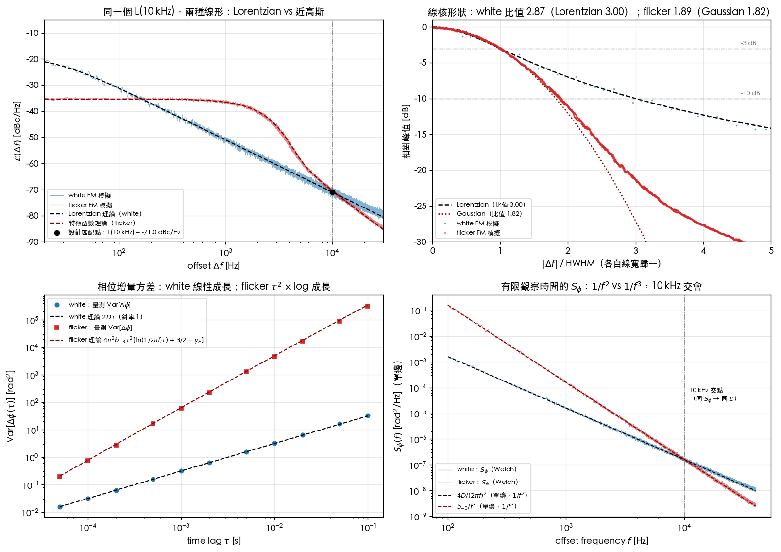
How to read the four panels:

• (a) top-left (PN view): the two simulated $\mathcal{L}(\Delta f)$ curves coincide at 10 kHz (black dot) at $-71$ dBc/Hz; moving toward the carrier, the white-noise curve climbs along the $-20$ dB/dec Lorentzian skirt and flattens at $\sim25$ Hz (HWHM); the flicker curve climbs more steeply along $-30$ dB/dec and already flattens at $\sim1.6$ kHz into a wide, flat Gaussian top. The black dashed line (Lorentzian) and the dark-red dashed line (numerical Fourier transform of the Step-4 characteristic function, no free parameters) sit on the two simulations respectively.
• (b) top-right (line-core shape, each normalized to its own HWHM): the white-noise point cloud hugs the Lorentzian reference line ($-10$ dB half-width at $3\times$ HWHM); the flicker point cloud hugs the Gaussian reference line ($-10$ dB half-width at $1.82\times$ HWHM), with the tail slightly above the pure Gaussian — exactly the log correction (theoretical ratio 1.86).
• (c) bottom-left (increment variance): the white-noise measured points fall on $2D\tau$ with slope 1; the flicker measured points fall on $4\pi^2b_{-3}\tau^2[\ln(1/2\pi f_l\tau)+3/2-\gamma_E]$ with slope $\approx2$ (dashed line, no free parameters).
• (d) bottom-right (finite-observation-time $S_\phi$): Welch applied directly to the nonstationary $\phi(t)$ — precisely Part B's "conditional spectrum" — yields a clean $1/f^2$ (on the single-sided theory $4D/\Delta\omega^2$) and $1/f^3$ (on $b_{-3}/f^3$), crossing at 10 kHz.

Core Python and actual run output (full script: simulations/lab_29_flicker_lineshape.py, run with PYTHONPATH=<project-root> python3 simulations/lab_29_flicker_lineshape.py; shared simulations/common/plot_utils.py, noise_utils.py):

# Matched design: K = 4D * f_match, so both oscillators have the same S_phi at f_match (hence the same L)
D  = 50.0 * np.pi          # white FM: Var[dphi] = 2 D |t|  [rad^2/s]
K  = 4 * D * 1.0e4         # flicker FM: S_phidot = K/f     [rad^2/s^2]
B3 = K / (4 * np.pi**2)    # S_phi = B3 / f^3               [rad^2 Hz^2]

print(f"{cal_first:.3f}")   # -> 0.986 (synthesis calibration: measured S_phidot·f ÷ K, near 1 kHz)
print(f"{L10_w:.1f}")       # -> -70.9 (white measured L(10 kHz); theory -71.0, time-domain /2 convention)
print(f"{L10_f:.1f}")       # -> -70.4 (flicker measured L(10 kHz); exact-lineshape theory is also -70.4, see below)
print(f"{r_onesided:.3f}")  # -> 1.001 (single-sided S_phi(10 kHz) ÷ (4D/Δω²): pins down "single-sided is 4D")
print(f"{fwhm_w:.1f}")      # -> 49.9 (white linewidth FWHM [Hz], theory D/π = 50.0)
print(f"{fwhm_f:.0f}")      # -> 3067 (flicker linewidth FWHM [Hz], 6-record ensemble; theory 3176)
print(f"{fwhm_f/fwhm_w:.1f}")  # -> 61.4 (same L(10 kHz), yet linewidths differ by 61x!)
print(f"{ratio_w:.2f}")     # -> 2.87 (white −10dB/−3dB half-width ratio; Lorentzian theory 3.00)
print(f"{ratio_f:.2f}")     # -> 1.89 (flicker half-width ratio; Gaussian 1.82, theory with log correction 1.86)
print(f"{rms_w:.2f}")       # -> 0.24 (white rms error of Lorentzian fit [dB], ±4 HWHM: agrees)
print(f"{rms_f:.2f}")       # -> 4.37 (flicker rms error of Lorentzian fit [dB]: clear deviation)
print(f"{popt_w[1]:.1f}")   # -> 25.0 (white fitted HWHM [Hz], theory D/2π = 25.0)
print(f"{r_th_f:.2f}")      # -> 1.86 (half-width ratio of the characteristic-function theory line)
print(f"{2*hw_th_f[0.5]:.0f}")  # -> 3176 (characteristic-function theoretical linewidth [Hz]; Gaussian freezing approximation 3233)
print(f"{10*np.log10(L_th_f_10k):.1f}")  # -> -70.4 (exact lineshape at 10 kHz: 0.6 dB above the pure 1/f³ skirt)
print(f"{slope_w/(2*D):.3f}")  # -> 1.010 (white measured Var/τ ÷ 2D: linear growth ✓)
print(f"{var_f[i1ms]/var_f_cf[i1ms]:.3f}")   # -> 0.957 (flicker Var(1 ms) ÷ closed form)
print(f"{var_f_cf[i10ms]/var_f_ex[i10ms]:.3f}")  # -> 1.000 (closed form ÷ exact discrete sum: derivation correct)
print(f"{r_cut:.2f}")       # -> 1.92 (cutoff experiment: ratio of Var(10 ms) for f_l=1/32 Hz vs 1 Hz, measured)
print(f"{r_cut_th:.2f}")    # -> 2.09 (same, exact theory: the cutoff enters via ln(f_l))

Three numbers worth pausing on:

1. $-70.4$ vs $-71.0$ (flicker's 0.6 dB): the flicker line converges to the $1/f^3$ skirt only for $\Delta f\gg$ linewidth; 10 kHz is only $\approx3\times$ HWHM, and the exact lineshape (numerical Fourier transform of the characteristic function) predicts $-70.4$ in the first place — measurement and exact theory agree completely; what deviates is the "pure-skirt approximation". This also quantifies how far "offset $\gg$ linewidth" really needs to be: at $3\times$ HWHM the error is still 0.6 dB.
2. The $61.4$× linewidth ratio: the same datasheet number $\mathcal{L}(10\,\text{kHz})=-71$ dBc/Hz can hide linewidths nearly two orders of magnitude apart. A single-point $\mathcal{L}$ does not determine the linewidth; the slope (noise color) does.
3. $1.92$ vs $2.09$ (cutoff experiment): moving the synthesis cutoff from $1/32$ Hz to 1 Hz nearly halves the phase variance at $\tau=10$ ms — the variance really does remember $f_l$ ($\ln f_l$ enters); the measurement is slightly below theory because of slow-component fluctuations across the 6 records (single-record linewidth spread $2944\pm142$ Hz vs. ensemble 3067 Hz) — itself a hands-on exhibit of Part B.

Toy-model honesty note: lab_29 synthesizes "phase → cosine" directly, with no amplitude dynamics and no transistors; it verifies the mathematics of Steps 1–4, not any particular circuit.

---

Part B: nonstationarity — $S_\phi$ strictly does not exist, so what does the instrument measure?

Step 5: the free-running $\phi(t)$ is not a stationary process

Wide-sense stationarity requires two things: a mean that does not change with time, and an autocorrelation $R_\phi(t_1,t_2)$ that depends only on $\tau=t_2-t_1$. For a white-noise-driven Wiener phase started at $t=0$ ($\phi(0)=0$), compute $R_\phi$ step by step:

(i) Take $t_2\ge t_1$ and split $\phi(t_2)=\phi(t_1)+\Delta$, where $\Delta=\phi(t_2)-\phi(t_1)$ is the noise integral over the interval $(t_1,t_2]$, independent of $\phi(t_1)$ (white noise is uncorrelated across disjoint intervals; for Gaussians, uncorrelated = independent).

(ii)

$$R_\phi(t_1,t_2)=\big\langle\phi(t_1)\,[\phi(t_1)+\Delta]\big\rangle =\big\langle\phi(t_1)^2\big\rangle+\underbrace{\langle\phi(t_1)\rangle\langle\Delta\rangle}_{=0} =2D\,t_1 .$$

General form (no ordering assumed):

$$\boxed{\ R_\phi(t_1,t_2)=2D\min(t_1,t_2)\ }$$

• This is not a function of $\tau$ — it depends on absolute time (how long since power-up). Moreover $\operatorname{Var}[\phi(t)]=2Dt\to\infty$: unbounded variance. Both violate stationarity.
• Consequence: the Wiener–Khinchin theorem (stochastic_noise_basics) presupposes stationarity. So "$S_\phi(f)$" as a stationary PSD strictly does not exist — expressions like $S_\phi=2D/\Delta\omega^2$ cannot be read literally by definition. Flicker FM is worse: even the increment variance needs $f_l$ to be finite (Step 3).
• But the increments are stationary: $\operatorname{Var}[\Delta\phi(\tau)]=2D|\tau|$ is independent of $t_0$ (Step 1 (i)). This is why [P2] describes ring jitter in increment language, $\sigma_{\Delta t}=\kappa\sqrt{\Delta t}$ ([P2] Eq.(8), p.792) — increment statistics are well defined, the PSD is not. Time-domain jitter language is, mathematically, more fundamental than "$S_\phi$".

Step 6: what does exist is the spectrum of $V(t)$ (the [E2] Demir view)

Although $\phi$ diverges, $V(t)=\cos(\omega_0t+\phi(t))$ is bounded, and its statistics converge to stationary:

• The divergence of the "absolute" phase does not matter — $V$ only sees $\phi\bmod 2\pi$, and the $\bmod 2\pi$ distribution of a random walk tends to uniform over time (the initial phase is forgotten).
• The autocorrelation retains only the phase difference: $\langle V(t)V(t+\tau)\rangle\to\tfrac12\cos(\omega_0\tau)E(\tau)$ (the Step-1 computation of lorentzian_linewidth, which uses precisely the stationary increment $\Delta\phi$) — depends only on $\tau$ ✓.

This is one of the core points of [E2] A. Demir, A. Mehrotra, and J. Roychowdhury, IEEE TCAS-I 47(5):655–674, 2000 (not among the five source PDFs, DOI 10.1109/81.847872): the output of a noisy oscillator converges to a stationary process, whose spectrum (a Lorentzian under white noise) is a rigorously well-defined object — and it is exactly what the spectrum analyzer measures. Part A of this page merely runs the same machinery with flicker's $\operatorname{Var}(\tau)$; the lineshape changes from Lorentzian to near-Gaussian, but "$V$ is stationary and its spectrum is well defined" is unchanged (flicker needs the $f_l$ cutoff to make $\dot\phi$ stationary).

One table for "what exists, and who measures it":

Object	Strictly exists?	Who measures it
the sample path $\phi(t)$	✓ (but nonstationary, unbounded walk)	nobody measures it directly (an infinite-range phase meter does not exist)
$S_\phi(f)$ as a stationary PSD	✗ (the Wiener–Khinchin premise fails)	— (a convenient notation; see Step 7)
increment statistics $\operatorname{Var}[\Delta\phi(\tau)]$	✓ (white: inherently; flicker: needs $f_l$)	time-interval analyzers / jitter measurement ([P2]'s $\kappa\sqrt{\Delta t}$), allan_variance
finite-observation spectrum $S_\phi^{(T)}(f)$, $f\gg1/T$	✓ (expectation well defined, converges)	phase-noise analyzer (phase discriminator + FFT; the PLL eats the walk below the loop bandwidth) — the Welch of lab_29 panel (d) is exactly this
$S_V(f)$ (the PSD of $V(t)$)	✓ ($V$ stationary, [E2])	spectrum analyzer, directly (linewidth, lineshape, and $\mathcal{L}$ are all read from it)
$\mathcal{L}(\Delta f)=\tfrac12S_\phi$	✓ when $\Delta f\gg$ linewidth (and $\gg1/T$)	the number on the datasheet

Step 7: reconciliation — what this site's $S_\phi$ formulas actually measure

So what do the pagefuls of $S_\phi$ and $\mathcal{L}$ formulas on this site (and in [P1]) mean? They are conditional spectra at finite observation time: take a record of length $T$ (or let the PLL/instrument subtract the slow drift), and do spectral estimation on "the increments that look stationary within this record". One can show (and lab_29 panel (d) demonstrates numerically) that for $f\gg1/T$ the expectation converges to

$$S_\phi^{(T)}(f)\ \xrightarrow[f\gg1/T]{}\ \frac{4D}{(2\pi f)^2}\ \text{（單邊，white FM）},\qquad \frac{b_{-3}}{f^3}\ \text{（flicker FM）},$$

with measured ÷ theory $=1.001$ (10 kHz; see the marker above). So every $S_\phi$ formula on this site is rigorously usable in the range $\Delta f\gg\max(1/T,\ \text{線寬})$; where they fail is precisely the "spurious divergence" region of lorentzian_linewidth — for $\Delta f\lesssim$ linewidth you must switch to reading $S_V$ (the Lorentzian / near-Gaussian lineshape). The two descriptions splice seamlessly over their common range of validity (Part A's 0.6 dB exercise quantifies the splice point).

Flicker adds one more twist (this page's own lesson): because $f_l$ enters the variance through $\ln$, "finite observation" leaves a logarithmic afterimage on flicker forever — lab_29's cutoff experiment ($f_l$ moved from $1/32$ Hz to 1 Hz halves $\operatorname{Var}(10\,\text{ms})$) and the single-record linewidth spread ($2944\pm142$ Hz, 6 records of only 32 s each) are direct displays of it. In practical language: for a flicker-dominated oscillator, the "linewidth" and the close-in integrated jitter are (weak) functions of "how long you measure"; quote the observation time / measurement bandwidth alongside the number — which is also why allan_variance exists (flicker FM shows up as a clean plateau on ADEV, well defined without any $f_l$). For the textbook treatment of this viewpoint see Rubiola 2009 (cited above, external literature).

Applicability and failure conditions

Condition	When it holds	What happens when it fails
$\Delta\phi$ Gaussian	characteristic function $E=e^{-\operatorname{Var}/2}$ exact (synthesized noise, small-signal linear accumulation)	strong nonlinearity / large injection makes $\Delta\phi$ non-Gaussian; the lineshape departs from both families on this page
$2\pi f_l\tau\ll1$	the $t^2\log$ closed form holds (error $O((f_l\tau)^2)$)	for $\tau\gtrsim1/f_l$ variance growth slows and the envelope tail deviates
pure flicker-FM segment dominates	near-Gaussian line core, ratio $\approx1.86$	with white FM mixed in, the outer region reverts to a Lorentzian skirt; the lineshape is a convolution of both families ([E3], Demir 2002)
$\Delta f\gg$ linewidth	$\mathcal{L}=\tfrac12S_\phi$ usable (still 0.6 dB off at $3\times$HWHM)	near the linewidth you must read the $S_V$ lineshape instead
observation time $T\gg1/\Delta f$	the conditional spectrum $S_\phi^{(T)}$ converges and matches the formulas	records too short: spectral-estimation bias plus flicker slow components that do not self-average (single-record linewidth spread)
amplitude stable (tracking phase only)	a single parameter ($D$ or $b_{-3}$) describes the lineshape	with strong AM–PM, amplitude noise must be modeled as well

Corresponding papers and equations

• The $1/f^2$, $1/f^3$ inputs to $S_\phi$: [P1] Eq.(21), p.185 (white); [P1] Eq.(22)–(23), p.185 (flicker upconversion, the ISF origin of $b_{-3}$, with the SSB bookkeeping note).
• Increment language: [P2] Eq.(8), p.792 ($\sigma_{\Delta\phi}=\kappa\sqrt{\Delta t}$, phase increments), Eq.(12), p.793 ($\kappa=\frac{\Gamma_{rms}}{q_{max}}\sqrt{\tfrac12\overline{i_n^2}/\Delta f}$, no $\omega_0$) — precisely the engineering embodiment of this page's "the PSD does not exist, the increments do".
• External literature (none among the five source PDFs): [E2] Demir–Mehrotra–Roychowdhury 2000 ($V$ stationary, spectrum well defined; TCAS-I 47(5):655–674, DOI 10.1109/81.847872); [E3] Kärtner 1990 ($f^{-\alpha}$ lineshape; IJCTA 18(5):485–519); A. Demir, IEEE TCAS-I 49(12):1782–1791, Dec. 2002 (colored-noise phase diffusion); E. Rubiola, Phase Noise and Frequency Stability in Oscillators, Cambridge Univ. Press, 2009 (textbook treatment).

Worked example (with units, verifiable in one line)

Example (same $\mathcal{L}$, two linewidths): a 5 GHz oscillator measures $\mathcal{L}=-71.0$ dBc/Hz at 10 kHz offset (time-domain $/2$ convention). (a) If that offset lies in the $1/f^3$ segment, with low-frequency cutoff $f_l=0.0176$ Hz (the effective cutoff of a 32 s observation), find $b_{-3}$, $\operatorname{Var}[\Delta\phi(1\,\text{ms})]$, and the linewidth; (b) if it lies in the $1/f^2$ segment, find the linewidth. Compare the two.

(a) Flicker case, step by step:

1. Recover $S_\phi$. $\mathcal{L}_{\text{lin}}=10^{-71/10}=7.94\times10^{-8}\ /\text{Hz}$; $S_\phi(10\,\text{kHz})=2\mathcal{L}_{\text{lin}}=1.589\times10^{-7}\ \text{rad}^2/\text{Hz}$.
2. Read off $b_{-3}$. $b_{-3}=S_\phi f^3=1.589\times10^{-7}\times(10^4)^3=1.589\times10^{5}\ \text{rad}^2\text{Hz}^2$.
3. Variance ($\tau=1$ ms). $2\pi f_l\tau=2\pi\times0.0176\times10^{-3}=1.10\times10^{-4}$; the bracket $=\ln(1/1.10\times10^{-4})+1.5-0.5772=9.11+0.92=10.03$; $\operatorname{Var}=4\pi^2\times1.589\times10^5\times(10^{-3})^2\times10.03=6.27\times10.03\approx63.0\ \text{rad}^2$. — within 1 ms the phase has already spread by $\sqrt{63}\approx8$ rad: fully decohered (memory-loss time $\tau^\*\approx0.16$ ms).
4. Linewidth (Gaussian freezing approximation). $L^\*\approx12.1$ (evaluated at $\tau^\*$): $\Delta f_{3\mathrm{dB}}\approx2.355\sqrt{b_{-3}L^\*}=2.355\sqrt{1.589\times10^5\times12.1}\approx3.3\ \text{kHz}$ (exact numerical Fourier transform: $3.2$ kHz).

(b) White case, step by step: $b_{-2}=S_\phi f^2=1.589\times10^{-7}\times10^8=15.89\ \text{rad}^2\cdot\text{Hz}$; $\Delta f_{3\mathrm{dB}}=\pi b_{-2}=49.9\ \text{Hz}$ (equivalently $D=\pi^2b_{-2}=156.8\ \text{rad}^2/\text{s}$, $D/\pi=49.9$ Hz); $\operatorname{Var}(1\,\text{ms})=2D\tau=0.314\ \text{rad}^2$ — at 1 ms still coherent.

Comparison: the same $-71$ dBc/Hz@10 kHz — flicker linewidth $3.2$ kHz vs. white $50$ Hz (64×); 1 ms phase variance $63$ vs. $0.31\ \text{rad}^2$ (200×). A single-point $\mathcal{L}$ spec does not cap close-in behavior.

Dimension check: $[b_{-3}]=\text{rad}^2\text{Hz}^2$, $\sqrt{b_{-3}\cdot(\text{無因次})}=\text{rad}\cdot\text{Hz}\to$ (rad dimensionless) $\text{Hz}$ ✓; $[b_{-2}]=\text{rad}^2\text{Hz}$, $\pi b_{-2}$ is Hz ✓; $[4\pi^2b_{-3}\tau^2]=\text{rad}^2$ ✓.

import numpy as np
gE = 0.5772156649
L = 10**(-71/10); Sphi = 2*L
b3 = Sphi*1e4**3; b2 = Sphi*1e4**2
var_1ms = 4*np.pi**2*b3*1e-6*(np.log(1/(2*np.pi*0.0176*1e-3))+1.5-gE)
print(round(b3), round(var_1ms,1), round(np.pi*b2,1))   # -> 158866 63.0 49.9

Key takeaways

• The Lorentzian is exclusive to white FM: it is inherited from the linear growth $\operatorname{Var}[\Delta\phi]=2D|t|$.
• The universal engine: $\operatorname{Var}[\Delta\phi(\tau)]=2\int_0^\infty S_\phi^{\text{單邊}}(f)(1-\cos2\pi f\tau)\,df$ (increment high-pass kernel; single-sided bookkeeping — substituting the white $4D/\Delta\omega^2$ recovers $2D|t|$; lab_29 measures a ratio of 1.001).
• Flicker FM ($S_\phi=b_{-3}/f^3$, needs a low-frequency cutoff $f_l$): $\operatorname{Var}=4\pi^2b_{-3}\tau^2[\ln\frac{1}{2\pi f_l\tau}+\frac32-\gamma_E]$ — $t^2\times\log$ growth; $f_l$ enters only through $\ln$ (a 10× change shifts it by only $\ln10$).
• Characteristic function $E=e^{-\operatorname{Var}/2}$ ⇒ near-Gaussian envelope ⇒ near-Gaussian line core; linewidth $\approx2.355\sqrt{b_{-3}L^\*}$ ($\propto\sqrt{\text{噪}}$, i.e. the square root of the noise strength; for white noise it is $\propto$ noise strength).
• Shape fingerprint, the $-10$ dB / $-3$ dB half-width ratio: Lorentzian $3.00$, Gaussian $1.82$, flicker with log correction $1.86$ (lab_29 measures white $2.87$, flicker $1.89$; Lorentzian-fit rms error 0.24 vs 4.37 dB).
• The same $\mathcal{L}(10\,\text{kHz})=-71$ dBc/Hz: white-noise linewidth 50 Hz, flicker linewidth 3.1 kHz (61×) — single-point PN does not determine the linewidth; the noise color does.
• Free-running $\phi$: $R_\phi=2D\min(t_1,t_2)$, unbounded variance ⇒ nonstationary ⇒ $S_\phi$ as a stationary PSD strictly does not exist; what exists: increment statistics ([P2]'s $\kappa\sqrt{\Delta t}$), the finite-observation conditional spectrum (converging to this site's formulas for $f\gg1/T$), and the stationary $S_V$ ([E2] Demir; what the spectrum analyzer measures).
• Flicker's measured quantities (linewidth, close-in jitter) depend as $\ln$ on observation time / cutoff — quote the conditions with the number.

Further reading

• The full white-noise counterpart (this page's control group): lorentzian_linewidth
• Where $1/f^3$ comes from ($c_0$ upconversion, [P1] Eq.(22)–(24)): flicker_noise_upconversion, lab_07
• Stationarity, Wiener–Khinchin, ergodicity: stochastic_noise_basics
• The canonical time-domain characterization of flicker FM (ADEV plateau, no $f_l$ needed): allan_variance
• How instruments measure $\mathcal{L}$ (SA / discriminator / cross-correlation): measurement_and_spurs
• The bridge between jitter language and $S_\phi$: psd_phase_noise_jitter
• The end-to-end numerical chain (with a Lorentzian stop): capstone_lc_end_to_end
• Full citations for the external literature ([E2], [E3]): references