Phase-noise measurement and spurs

β: This English translation is in beta — the Traditional-Chinese original is the authoritative version.

Prerequisites: white_noise_to_phase_noise ($\mathcal{L}\approx\tfrac12 S_\phi$, the $1/f^2$ mid-band, useful for back-solving $S_i$), fourier_series_of_isf (the mechanism by which a spur is downconverted through the ISF's $n$-th harmonic $c_n$), symmetry (back-solving $c_0/c_1$ symmetry from the $1/f^3$ corner) | Next: real_oscillator_topologies, lorentzian_linewidth

The previous chapters carried phase noise from the ISF all the way to $\mathcal{L}(\Delta f)$ (SSB phase noise, units dBc/Hz) — all as "theoretical prediction." This page returns to the test bench and answers three questions that always come up in real measurement:

1. How do you measure $\mathcal{L}(f)$? Three mainstream methods — the spectrum analyzer (SA) direct method, the PLL/delay-line frequency discriminator (carrier-suppression method), and cross-correlation (correlating two independent channels to push the instrument floor down by a square root) — each with its own principle, pros/cons, and applicable range.
2. How do you distinguish a spur (spurious tone, a deterministic sideband) from random phase noise? One is a discrete tone (units dBc, not /Hz), the other a continuous spectrum (/Hz). They look different on the spectrum, have different causes, and need different countermeasures.
3. How do you read a real PN plot? Mark the $1/f^3$, $1/f^2$, and floor segments, the corners, and the spurs, then back out design information.

Physical intuition (conclusion first): the fundamental difficulty in measuring phase noise is that the device under test's (DUT's) phase jitter is tiny (often $-100$ to $-150$ dBc/Hz at 1 MHz offset), while your own instrument jitters too. So every method does the same thing: find a way to remove the tall, clean carrier tone, leaving only the faint noise skirt beside it, while making the measurement system's own noise floor lower than the DUT's. The three methods are three engineering approaches to "remove the carrier + push down the floor."

Honesty note: this page's measurement-instrument architectures and standards (PN spectrum analyzers, delay-line/PLL discriminators, cross-correlation analyzers — e.g. Keysight E5052B, R&S FSWP, Holzworth, etc.) are external engineering literature and instrument manuals, not among the five source PDFs. This page supplements with standard measurement theory and ties every result back to [P1]'s ISF framework. The underlying physics (carrier removal, PSD estimation, correlation averaging) is general DSP/communications knowledge; specific instrument models are used only as examples.

---

Part 1: three methods for measuring $\mathcal{L}(f)$

First, state clearly what we're measuring. Write the oscillator output as

$$v(t)=V_0\,\big[1+a(t)\big]\cos\!\big(\omega_0 t+\phi(t)\big),$$

where $a(t)$ is AM noise (amplitude noise) and $\phi(t)$ is PM noise (phase noise, this site's main subject). We want the single-sideband power spectrum of the phase part:

$$\mathcal{L}(\Delta f)\approx\tfrac12 S_\phi(\Delta f)\quad[\text{dBc/Hz}],$$

(small-angle approximation, canonical Eq.16; see white_noise_to_phase_noise). The three methods differ in "how cleanly $\phi(t)$ is separated from $v(t)$ without being contaminated by the instrument's own phase noise."

Method A: direct spectrum-analyzer method

Principle: connect the DUT directly to a spectrum analyzer and look at the power-spectrum skirt beside the carrier $f_0$. At offset $\Delta f$, resolution bandwidth $\text{RBW}$, the measured sideband power $P_{SSB}(\Delta f)$ relative to carrier power $P_{carrier}$, normalized to 1 Hz:

$$\mathcal{L}(\Delta f)=10\log_{10}\!\left(\frac{P_{SSB}(\Delta f)}{P_{carrier}}\right)-10\log_{10}(\text{ENBW}/1\,\text{Hz})\ +\ 2.5\,\text{dB}.$$

• The first term is "how many dB the sideband is below the carrier" (dBc).
• The second term normalizes the measurement bandwidth to per-Hz (using the equivalent noise bandwidth ENBW rather than the nominal RBW; e.g. for ENBW $\approx1$ kHz you subtract $10\log_{10}1000=30$ dB).
• The $+2.5$ dB is a common correction: a log detector combined with video/sample averaging underestimates Gaussian noise by about $2.5$ dB (Rayleigh-log bias), so about $2.5$ dB must be added back to recover the true noise power (external literature: Keysight/Agilent AN-1303 spectrum analysis basics). This is a toy/illustrative approximation; real instruments auto-correct this in their built-in PN measurement mode.

Unit check: $10\log_{10}(\text{dimensionless W/W})-10\log_{10}(\text{Hz})=\text{dBc}-\text{dB(Hz)}=\text{dBc/Hz}$ ✓.

Advantages:

• Fastest setup — a single SA does it; you also see spurs (discrete tones) and the broadband noise landscape at the same time.

Fatal drawback — the SA's own phase noise:

• What you measure is not the DUT's $S_\phi^{DUT}$, but the sum of the DUT's and the SA's local oscillator (LO) phase noise:

$$S_\phi^{meas}(\Delta f)=S_\phi^{DUT}(\Delta f)+S_\phi^{SA\,LO}(\Delta f).$$

As long as the DUT is cleaner than the SA's LO, what you measure is the SA itself — you're measuring the instrument, not the DUT.

• Also, the SA measures the sum of AM+PM; near the carrier PM usually dominates, but it cannot separate AM from PM.

Applicable range: when the DUT's phase noise is clearly worse than the SA's LO (e.g. measuring a noisy free-running ring VCO), or when you just need a quick look at spurs and the rough skirt shape. Not suitable for low-noise reference sources (OCXO, low-noise PLL), since you'll hit the SA floor.

Method B: PLL / delay-line frequency discriminator (carrier-suppression method)

The problem with the direct method is that "the big carrier tone is still there, and the small noise beside it is swamped by the instrument's dynamic range and LO noise." The idea of carrier suppression: first cancel the carrier term $\cos(\omega_0 t)$ with a phase detector, converting only $\phi(t)$ into a baseband voltage fed into a low-frequency FFT analyzer (whose floor is far below an RF SA's). There are two carrier-suppression methods:

B-1: PLL (phase-locked loop) method — lock to a clean reference

Feed the DUT and a cleaner reference source into a mixer (used as a phase detector), and use a PLL to lock the two at $90^\circ$ (quadrature). At quadrature the mixer output is linear in the phase difference:

$$v_{out}(t)=K_\phi\,\big[\phi_{DUT}(t)-\phi_{ref}(t)\big],$$

$K_\phi$ is the phase-detector gain (V/rad). The PLL loop bandwidth is set very low, so that at the offsets of interest $\phi_{ref}$ is tracked out by the loop, leaving only the DUT's phase fluctuation converted to voltage. FFT $v_{out}$ and divide by $K_\phi^2$ to get $S_\phi^{DUT}$.

• Advantages: the floor can be made extremely low (limited by the reference source, mixer, baseband amplifier), making it one of the gold-standard methods for low-noise sources; it naturally measures only PM (a mixer at quadrature is insensitive to AM).
• Drawbacks: needs a reference source cleaner than the DUT (the biggest pain point); requires locking, so the DUT must be stable enough; offsets below the PLL loop bandwidth get eaten by the loop and need loop-transfer correction.

B-2: delay-line frequency discriminator — using the DUT as its own reference

When you cannot find a cleaner reference source (e.g. measuring a source that is itself the best low-noise part available), use the DUT delayed by $\tau_d$ as its own reference. Split the signal into two paths, one through a delay line $\tau_d$, the other through a phase shifter tuned to quadrature, then into a mixer. The delay converts frequency fluctuation into a phase difference, which the mixer resolves. Its transfer function (converting frequency noise $S_{\Delta f}$ into output) is

$$\big|H(\Delta f)\big|^2=\big(2\pi\tau_d\big)^2\,\operatorname{sinc}^2(\Delta f\,\tau_d),\qquad \operatorname{sinc}(x)=\frac{\sin(\pi x)}{\pi x},$$

here $H$ maps frequency fluctuation $\delta f$ to output. The discriminator senses frequency fluctuation, and frequency is the derivative of phase, so the bridging relation between the frequency spectrum and phase spectrum is $S_{\delta f}(\Delta f)=\Delta f^2\,S_\phi(\Delta f)$ (each extra derivative adds one $\Delta f$ factor in the frequency domain). Substituting this back gives an extra $\Delta f^2$ in the denominator (i.e. $(2\pi\tau_d)^2\to(2\pi\,\Delta f\,\tau_d)^2$),

so

$$S_\phi(\Delta f)=\frac{S_{v}(\Delta f)}{K_\phi^2\,(2\pi\,\Delta f\,\tau_d)^2\,\operatorname{sinc}^2(\Delta f\,\tau_d)}.$$

• Physical meaning: the delay line converts frequency discrimination into phase, with sensitivity $\propto\tau_d$ — the longer the delay, the more sensitive.
• Drawback: sensitivity $\propto\tau_d$, but $\operatorname{sinc}$ has nulls at $\Delta f=k/\tau_d$ — too long a delay narrows the usable offset range and blinds the measurement at the nulls; the delay line itself has loss (attenuates the signal, raises the floor). It's a "sensitivity vs. frequency coverage" trade-off.
• Advantage: needs no external reference source, self-sufficient; good for measuring a source that is itself extremely clean, with no better reference available.

Unit check (delay-line): $S_v$ is $\text{V}^2/\text{Hz}$; dividing by $K_\phi^2$ ($\text{V}^2/\text{rad}^2$) gives $\text{rad}^2/\text{Hz}$; the denominator $(2\pi\Delta f\tau_d)^2$ is dimensionless, so overall $\text{rad}^2/\text{Hz}=S_\phi$ ✓.

Method C: cross-correlation — using square-root averaging to push down uncorrelated instrument floors

This is the signature technique of modern commercial PN analyzers (e.g. E5052B, FSWP, Holzworth), not among the five source PDFs, and belongs to external instrument literature. It addresses Method B's fundamental limitation: the measurement channel's own floor.

Core idea: split the same DUT's signal into two paths, each connected to a fully independent carrier-suppression + measurement channel (each with its own reference source/mixer/amplifier, whose floors are mutually uncorrelated). The two path outputs are

$$y_1(t)=\phi_{DUT}(t)+n_1(t),\qquad y_2(t)=\phi_{DUT}(t)+n_2(t),$$

where $\phi_{DUT}$ is the DUT phase shared by both paths (correlated), and $n_1,n_2$ are each channel's independent instrument floor (uncorrelated). Compute the cross-spectrum $S_{y_1 y_2}=\langle Y_1 Y_2^*\rangle$ of the two paths and average $M$ times:

$$S_{y_1 y_2}(\Delta f)=\underbrace{S_{\phi\phi}(\Delta f)}_{\text{correlated, retained}}+\underbrace{\frac{1}{\sqrt{M}}\big(\text{uncorrelated floor term}\big)}_{\text{drops with square root of averages}}.$$

• Key physics: the DUT phase is correlated across the two paths, so it adds coherently in the cross-correlation and is retained in full; the two channels' instrument floors are uncorrelated, so in the cross-correlation they behave as random phase and, after averaging over $M$ segments, converge as $1/\sqrt{M}$ (every 10× more averaging drops the floor by $5$ dB, i.e. $10\log_{10}\sqrt{10}=5$ dB).
• How much you can gain: relative to the single-channel floor, you can additionally lower it by

$$\Delta_{floor}=5\log_{10}M\ \text{[dB]}\quad(\text{5 dB per }\times10\text{ averaging}).$$

Dropping $20$ dB needs $M=10^4$ averages; beyond a certain point you're limited by residual correlation between channels (shared supply, reference distribution, thermal) and measurement time.

Advantages: the floor can be pushed lower than any single reference source — you can measure world-class low-noise sources; the same architecture can separate AM and PM simultaneously. Drawbacks: needs two independent sets of hardware, expensive; near the carrier needs heavy averaging, so measurement time is long ($M$ large); residual correlation sets a practical limit. Applicable range: measuring the lowest-noise sources (OCXO, low-noise synthesizers, integrated PLLs), the method of choice when you need to approach the physical floor limit.

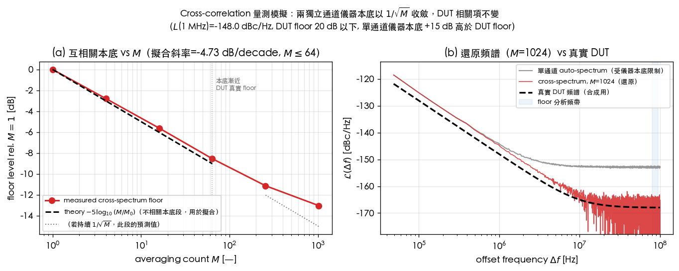
Method C simulation: two-channel cross-correlation squeezes the instrument floor by a square root

The $1/\sqrt{M}$ convergence above is only a verbal description; here is a reproducible numerical simulation that actually produces it, so you can see with your own eyes how "the single channel measures the instrument floor, while cross-correlation digs the true DUT floor back out" happens (full code: simulations/lab_35_xcorr_measurement.py; figure: static/figures/xcorr_floor.png).

Methodology walkthrough:

1. Synthesize a "true" DUT spectrum: use the site's canonical values (Example B: $q_{max}=1$ pC, $\Gamma_{rms}=0.5$; [P1] Eq.(21) gives $\mathcal{L}(1\text{ MHz})=-148.0$ dBc/Hz, i.e. $S_\phi(1\text{ MHz})=2\times10^{-14.8}=3.17\times10^{-15}$ rad²/Hz) as the $1/f^2$ mid-band, then add a white floor $20$ dB below it ($S_{DUT,floor}=3.17\times10^{-17}$ rad²/Hz) — an honest "two-segment" toy DUT spectrum: $1/f^2$ near the carrier, flattening far out. This is a known answer, so we can check whether the measurement method actually recovers it.
2. Add instrument white noise to two independent channels: $y_1(t)=\phi_{DUT}(t)+n_1(t)$, $y_2(t)=\phi_{DUT}(t)+n_2(t)$, $n_1\perp n_2\perp\phi_{DUT}$, each channel's floor set $15$ dB above the DUT floor ($S_{instr}=10^{1.5}\times S_{DUT,floor}\approx1.00\times10^{-15}$ rad²/Hz) — matching the comparison table's scenario where "single-channel floor $=$ DUT floor $+$ instrument floor."
3. Compute both spectra from the same data: the single-channel auto-spectrum $S_{yy}=\langle|Y_1|^2\rangle$ ($M$-segment averaged) and the cross-spectrum $S_{y_1y_2}=\langle Y_1Y_2^*\rangle$ (also $M$-segment averaged), with $M=1,4,16,64,256,1024$ (powers of 4).
4. In a high-offset band far from $f_{ref}$ ($80$–$95$ MHz, where the DUT's $1/f^2$ skirt has already decayed to below $1.5\%$ of the DUT floor and can be treated as "floor only"), measure how the cross-spectrum residual floor changes with $M$, and fit a straight line over $M\le64$ (where the residual floor is still clearly above the true DUT floor, i.e. "uncorrelated-noise-dominated"), comparing against the canonical slope $\Delta_{floor}=5\log_{10}M$.
5. At $M=1024$, compare the recovered spectrum against the true DUT spectrum: can cross-correlation dig out the DUT's true floor, which the single channel cannot resolve.

Key results (# -> marks program output):

$M$	Cross-spectrum residual floor [rad²/Hz]	Rel. $M{=}1$ [dB]	Theory $-5\log_{10}M$ [dB]
1	$8.38\times10^{-16}$	$0.00$	$0.00$
4	$4.40\times10^{-16}$	$-2.79$	$-3.01$
16	$2.30\times10^{-16}$	$-5.62$	$-6.02$
64	$1.17\times10^{-16}$	$-8.55$	$-9.03$
256	$6.43\times10^{-17}$	$-11.15$	$-12.04$
1024	$4.15\times10^{-17}$	$-13.05$	$-15.05$

Fitting a slope over $M\le64$ (where the uncorrelated residual is still clearly above the DUT floor): fitted slope $=-4.73$ dB/decade, vs. theory $-5.00$ dB/decade, match $=0.946$ (# -> slope match: fitted/theory = 0.9463) — with finite samples ($\sim300$ independent frequency bins, averaged over 8 independent realizations), the $1/\sqrt{M}$ law is cleanly verified.

By $M=256$ and $1024$, the numbers start to deviate from the theory line ($-11.15$, $-13.05$ dB, "shallower" than the theoretical $-12.04$, $-15.05$ dB) — this is not an error, it is physics: because the simulation only sweeps $M$ up to $1024$ ($\sqrt{M}$ is only $32\times$, about $15$ dB of possible improvement), and the single-channel margin is also set at $15$ dB, the two are of comparable magnitude, so by $M=1024$ the residual uncorrelated floor $S_{instr}/\sqrt{M}$ has approached (rather than fallen far below) the true DUT floor $S_{DUT,floor}$, and the residual curve bends toward the true floor instead of continuing to follow the pure $1/\sqrt{M}$ line — this is the signature of cross-correlation succeeding at pushing the floor down near the DUT's true value, not a failure.

Recovery performance (at $M=1024$, see panel (b) below):

• In the DUT floor region (near $90$ MHz): the true value is $\mathcal{L}=-167.95$ dBc/Hz; the single channel measures $-152.74$ dBc/Hz (masked by the instrument floor, off by $15.2$ dB — what it measures is really the instrument); cross-correlation ($M=1024$) measures $-166.15$ dBc/Hz, only $+1.79$ dB off (# -> residual error at DUT floor after M=1024 averaging: +1.79 dB) — the DUT's true floor, completely hidden under the instrument floor, is dug back out almost fully by correlating two independent channels and averaging.
• In the $1/f^2$ mid-band ($1$ MHz): the DUT's own signal is large enough that both the single channel and cross-correlation are close to the true value ($-147.80$ dBc/Hz true vs. $-143.87$ single-channel, $-144.43$ cross-correlation) — cross-correlation isn't really needed here; the point of the demonstration is the floor (far offset), not where the signal is already strong.

Honesty note: what is verified here is only the statistical/DSP mechanism behind cross-correlation (the $1/\sqrt{M}$ convergence itself is a property of general complex-Gaussian statistics, not content from this site's five source PDFs, and not ISF physics), and in the model the two channels' instrument floors are set to be perfectly uncorrelated. On a real instrument, $M\to\infty$ cannot push the floor down without limit — residual inter-channel correlation (shared reference clock distribution, shared supply/ground, thermal coupling) sets a physical floor not modeled in this simulation (external engineering literature, not among the five source PDFs; the simulation above only demonstrates the idealized $1/\sqrt{M}$ mechanism and one realistic finite-$M$ outcome, not that the floor can be pushed arbitrarily low).

Comparison of the three methods

Method	Carrier-suppression mechanism	External reference needed?	Floor (relative)	Main limitation	Best for
A. Direct SA method	None (looks directly at the skirt)	No	High (= SA's own LO)	Measures the SA itself; can't separate AM/PM	Quick spur look / noisy DUT
B-1. PLL lock	Mixer + PLL lock to quadrature	Needs a cleaner reference	Low	Limited by reference source; near-carrier eaten by loop	Low-noise source (with a good reference available)
B-2. Delay-line	Self-delay $\tau_d$ as reference	No (self-referenced)	Medium–low	$\operatorname{sinc}$ nulls, delay loss	Clean source with no better reference
C. Cross-correlation	Two paths each carrier-suppressed + cross-correlated	Depends on architecture (often internal reference)	Lowest ($\propto1/\sqrt{M}$)	Expensive, slow, residual correlation limits	World-class low-noise source

One-line summary: Method A measures "DUT plus instrument"; Method B replaces the instrument's LO with either a good reference or its own delay; Method C accepts that "every channel has a floor," but uses correlation across two independent channels to square-root-kill the uncorrelated floor.

---

Part 2: spurs (deterministic sidebands) vs. random phase noise

A measured PN plot commonly shows two completely different things superimposed, which newcomers easily confuse. First, pin down the definitions:

Item	Random phase noise	Spur (spurious tone)
Nature	Random (stochastic) process	Deterministic sine tone
Spectral appearance	Continuous skirt	Discrete single spike
Units	/Hz (dBc/Hz, power density)	dBc (total power ratio, no /Hz)
Vs. RBW	Measured dBc/Hz does not change with RBW (already normalized)	Spike height (dBc) does not change with RBW; but "appears" to widen/narrow with RBW
Cause	Device thermal/flicker noise, upconverted via ISF	Reference leakage, supply ripple, external injection, and other periodic disturbances
Countermeasure	Improve ISF symmetry, increase $q_{max}$, lower device noise	Find the interferer, isolate/filter/shield

2.1 Why the units are so different: density vs. total power

Random PN is a power density: phase is a continuous random process, so its power is spread across the frequency axis; only "power per Hz" is meaningful — hence dBc/Hz. Double the measurement bandwidth RBW and the measured noise power doubles too, but once normalized to per-Hz the number does not change.

A spur is the total power of a discrete tone: a deterministic sine wave's entire power sits at a single frequency, with theoretically zero bandwidth. Its "density" is infinite (meaningless), so only the total power relative to the carrier, in dBc, is reported — no /Hz. Increasing RBW does not change its dBc value (all the power is in that one spike); it just looks "fatter."

Measurement trap: on a PN analyzer, the continuous background is plotted in dBc/Hz, but if a spur is also plotted as "the density at the current RBW," it will drift up and down as you change RBW — this is an artifact. The correct approach is for the instrument to flag spurs separately in dBc (integrated total power). Discriminating rule: change the RBW setting and remeasure — the random PN's dBc/Hz number does not move, but the spur's "dBc/Hz reading" will change (because it is not a density). Whichever number moves is the spur.

2.2 Typical causes of spurs and countermeasures

Spur frequency location	Typical cause	Physical mechanism (tied to ISF)	Countermeasure
$f_{ref}$ and its harmonics (reference spur)	PLL reference leakage, charge-pump mismatch, PFD dead zone	Periodic disturbance at the reference frequency, upconverted to near the carrier via the ISF's $n$-th harmonic	Reduce CP leakage/mismatch, optimize PFD, strengthen loop-filter rejection
Supply ripple frequency (e.g. $50/60$ Hz, switching supply $\sim$ hundreds of kHz)	Periodic ripple on supply/ground coupling into tank/tail	Periodic supply disturbance → upconverted via ISF's $c_0/c_n$	Regulator/LDO decoupling, layout isolation, lower PSRR sensitivity
Nearby strong-signal frequency	External RF injection, injection pulling	Injected signal pulls the oscillator (see injection locking)	Shielding, isolation, larger tank $Q$ to resist pulling
Digital clock and its harmonics	Digital aggressor coupling via substrate/supply	Periodic digital edges, upconverted via ISF	Guard rings, separate supply domains, timing offset

The key insight tying this back to the ISF: a deterministic injected single tone landing at $n\omega_0+\Delta\omega$ (near the $n$-th harmonic) gets downconverted by the ISF's $n$-th Fourier coefficient $c_n$ to $\Delta\omega$ beside the carrier, producing a spur ([P1] Eq.(16/17), p.183, the single-tone version; see fourier_series_of_isf):

$$\phi(t)\approx\frac{I_0\,c_n\sin(\Delta\omega t)}{2q_{max}\,\Delta\omega}.$$

• This uses the same ISF mechanism as random PN — the only difference is "whether the source is a deterministic single tone (→ spur) or white noise (→ continuous spectrum)."
• Design implication: if a spur lands near the $n$-th harmonic, lowering the ISF's $c_n$ (by improving waveform symmetry) suppresses that spur too — the same knob set as for lowering random PN.

2.3 Distinguishing them on a spectrum (operational procedure)

1. Look at the shape: continuous skirt = random PN; isolated spike = spur.
2. Change the RBW and re-weight: dBc/Hz unchanged is PN; a reading that changes with RBW is a spur.
3. Check repeatability: a spur's frequency is fixed (locked to $f_{ref}$, ripple frequency, etc.); toggling nearby equipment (power supplies, nearby transmitters) makes the spur move/disappear; random PN is intrinsic to the DUT and cannot be switched off.
4. Integrate power: integrating a spur gives a fixed dBc (independent of RBW); integrating PN gives jitter (see numerical_feeling).

---

Part 3: how to read a real PN plot

Bringing the first two parts together: given a plot of $\mathcal{L}(\Delta f)$ vs. offset (log–log), how do you read out design information? A typical free-running oscillator's PN plot consists of three sloped segments plus some spurs.

3.1 Three slopes and two corners

Region	Slope	Physical origin	Corresponding equation
Close-in (nearest the carrier)	$-30$ dB/dec ($1/f^3$)	Device flicker ($1/f$) noise upconverted via $c_0$ (ISF DC asymmetry)	[P1] Eq.(23), p.185
Mid-band	$-20$ dB/dec ($1/f^2$)	White noise through the phase integrator $1/\omega^2$	[P1] Eq.(21), p.185
Floor (farthest out)	$0$ dB/dec (flat)	White noise floor of the measurement system/buffer	—

Two turning points:

• The $1/f^3$ corner $\Delta f_{1/f^3}$: where $1/f^3$ crosses $1/f^2$. From [P1] Eq.(24), p.185:

$$\Delta\omega_{1/f^3}=\omega_{1/f}\cdot\frac{c_0^2}{2\,\Gamma_{rms}^2}\approx\omega_{1/f}\left(\frac{c_0}{c_1}\right)^2.$$

It reflects ISF symmetry: the smaller $c_0$ (ISF DC component) is — the more symmetric the waveform — the closer this corner sits to the carrier and the narrower the $1/f^3$ region — this is the quantitative basis for "why pursue a symmetric waveform" (see symmetry).

• The noise-floor corner $\Delta f_{floor}$: where $1/f^2$ crosses the flat floor. It is usually the floor of the measurement system or output buffer, not necessarily intrinsic to the oscillator — when reading a plot, first confirm whether the floor is the DUT's or the instrument's (using cross-correlation from Part 1 to push down the instrument floor, so you can see the DUT's real floor).

3.2 Back-solving design information (a reading checklist)

• Height and width of the $1/f^3$ region → device flicker magnitude ($\omega_{1/f}$) and ISF symmetry ($c_0$). If close-in performance is poor → switch to a lower-flicker device, symmetrize the waveform/layout, use a tail filter to suppress $c_0$.
• Height of the $1/f^2$ region → $\Gamma_{rms}^2/q_{max}^2 \cdot S_i$. If too high → increase swing ($q_{max}$), lower device white noise, suppress $\Gamma_{rms}$ (see tank_swing). A $20$ dB improvement per decade in the $1/f^2$ region is a physical law — if the slope is off, suspect a measurement error.
• Floor height → confirm whether it is the DUT or the instrument. If it's the buffer, increase carrier power or switch to a lower-noise buffer.
• Spurs → identify each one: $f_{ref}$? ripple? injection? Apply the countermeasures in the 2.2 table respectively.

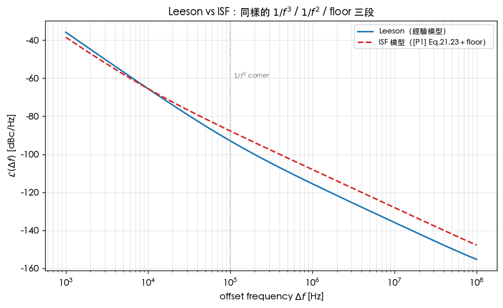
This whole PN plot picture — the Leeson model and the ISF model produce the same three-segment broken line — this site's derivation_leeson and the leeson_vs_isf figure overlay both models; the three segments ($1/f^3$, $1/f^2$, floor) and corners line up exactly. The only difference is that the ISF explains each segment's constant in terms of $\Gamma_{rms}$, $c_0$, $q_{max}$, while Leeson uses the empirical $Q$, $F$.

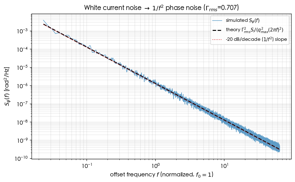
The simulated white-noise → $1/f^2$ spectrum below is exactly what the $-20$ dB/dec mid-band segment in the figure above looks like in isolation (toy model, see lab_06):

---

Numerical examples: back-solving design from plot readings (worked examples)

The two problems below follow the strict format: problem (given plot readings) → step-by-step substitution (with units) → result → dimension check → one-line Python check. Using the same canonical values as Section 8 ($q_{max}=1$ pC, $\Gamma_{rms}=0.5$, $f_0=5$ GHz).

Example 1 (back-solving the equivalent white noise $S_i$ from a $1/f^2$ reading): on a PN plot, the mid-band ($1/f^2$ region) reads $\mathcal{L}(1\,\text{MHz})=-148.0$ dBc/Hz. Given $q_{max}=1$ pC, $\Gamma_{rms}=0.5$. Back-solve the equivalent white-noise current PSD $S_i=\overline{i_n^2}/\Delta f$.

Step-by-step substitution (inverting [P1] Eq.(21), p.185):

1. Convert dBc/Hz to linear: $10^{\mathcal{L}/10}=10^{-14.8}=1.585\times10^{-15}$ (dimensionless per-Hz).
2. Offset angular frequency: $\Delta\omega=2\pi\times10^{6}=6.283\times10^{6}$ rad/s, $\Delta\omega^2=3.948\times10^{13}$ rad²/s².
3. Eq.(21) is $\mathcal{L}=\dfrac{\Gamma_{rms}^2}{q_{max}^2}\cdot\dfrac{S_i}{4\Delta\omega^2}$; inverting,

$$S_i=\mathcal{L}_{lin}\cdot\frac{4\,\Delta\omega^2\,q_{max}^2}{\Gamma_{rms}^2}.$$

4. Substitute: $S_i=1.585\times10^{-15}\times\dfrac{4\times3.948\times10^{13}\times(10^{-12})^2}{0.25}$ $=1.585\times10^{-15}\times\dfrac{1.579\times10^{14}\times10^{-24}}{0.25}=1.585\times10^{-15}\times6.317\times10^{-10}\approx1.0\times10^{-24}$.

Result: $S_i\approx1.0\times10^{-24}\ \text{A}^2/\text{Hz}$ — exactly recovering the canonical Example B input value (self-consistent).

Dimension check: $\mathcal{L}_{lin}$ (per-Hz $=$ s) $\times\dfrac{(\text{rad/s})^2\cdot\text{C}^2}{1}=\text{s}\cdot\dfrac{\text{C}^2}{\text{s}^2}=\dfrac{\text{C}^2}{\text{s}}=\dfrac{(\text{A}\cdot\text{s})^2}{\text{s}}=\text{A}^2\cdot\text{s}=\text{A}^2/\text{Hz}$ ✓.

import numpy as np
L_dbc, gamma_rms, qmax = -148.0, 0.5, 1e-12
dw = 2*np.pi*1e6
Si = 10**(L_dbc/10) * (4*dw**2*qmax**2) / gamma_rms**2
print(f"{Si:.3e} A^2/Hz")   # -> 1.000e-24 A^2/Hz

Example 2 (back-solving ISF symmetry $c_0/c_1$ from the $1/f^3$ corner): the plot reads a device flicker corner $f_{1/f}=1\,\text{MHz}$ ($\omega_{1/f}=2\pi\times10^6$), and the $1/f^3$–$1/f^2$ crossover on the PN plot appears at $\Delta f_{1/f^3}=100\,\text{kHz}$. Back-solve the ISF's $c_0/c_1$ ratio and assess waveform symmetry.

Step-by-step substitution (using [P1] Eq.(24), p.185's approximation $\Delta\omega_{1/f^3}\approx\omega_{1/f}(c_0/c_1)^2$):

1. Invert: $\left(\dfrac{c_0}{c_1}\right)^2=\dfrac{\Delta\omega_{1/f^3}}{\omega_{1/f}}=\dfrac{2\pi\times10^5}{2\pi\times10^6}=\dfrac{10^5}{10^6}=0.1$.
2. Take the square root: $\dfrac{c_0}{c_1}=\sqrt{0.1}\approx0.316$.

Result: $c_0/c_1\approx0.32$ — the ISF's DC component is about one-third of its first harmonic, indicating "moderate symmetry."

Design implication: $c_0\neq0$ means the waveform/layout still has asymmetry, with appreciable $1/f^3$ upconversion still present. If further symmetrizing the waveform lowers $c_0$ by another $\times0.3$ ($c_0/c_1\to0.1$), the corner drops from $100$ kHz to $\Delta f_{1/f^3}=\omega_{1/f}(0.1)^2=1\,\text{MHz}\times0.01=10\,\text{kHz}$ — the close-in $1/f^3$ region shrinks 10×, substantially improving near-carrier noise (see symmetry, flicker_noise_upconversion).

Dimension check: $\Delta\omega_{1/f^3}/\omega_{1/f}$ is rad/s ÷ rad/s $=$ dimensionless; $(c_0/c_1)^2$ is also dimensionless ✓.

import numpy as np
w_1f = 2*np.pi*1e6           # device flicker corner
dw_1f3 = 2*np.pi*1e5         # 1/f^3 corner read off the plot
c0_over_c1 = np.sqrt(dw_1f3/w_1f)
print(round(c0_over_c1, 3))  # -> 0.316

---

Validity and breakdown conditions

Condition	Holds when	What happens when it breaks down
Measurement-system floor $\ll$ DUT noise	You measure the DUT	You measure the instrument itself (easiest pitfall of the direct SA method) → switch to PLL/cross-correlation
Small-angle PM ($\phi\ll1$ rad)	$\mathcal{L}\approx\tfrac12 S_\phi$	Large phase excursions need the rigorous PM spectrum; near-carrier Lorentzian (see lorentzian_linewidth)
Noise source is stationary white/flicker	Clean three-segment broken line	Cyclostationarity, injection pulling break the clean broken line
Spur is a deterministic periodic source	dBc is fixed, can be identified individually	Random burst/intermittent interference is hard to describe with dBc
Floor is intrinsic to the DUT	Floor reflects the buffer/source	Usually it's the instrument floor; cross-correlation is needed to see the true floor

Correspondence with papers/equations

• Spur downconversion mechanism (single-tone version): [P1] Eq.(16/17), p.183 (see fourier_series_of_isf).
• $1/f^2$ mid-band: [P1] Eq.(21), p.185; $1/f^3$ close-in: [P1] Eq.(23), p.185; $1/f^3$ corner: [P1] Eq.(24), p.185.
• $\mathcal{L}\approx\tfrac12 S_\phi$ (small-angle PM): canonical Eq.16.
• Full three-segment picture and Leeson comparison: derivation_leeson, [E1] Leeson 1966 (not among the five source PDFs).
• Measurement instruments/standards (SA, delay-line/PLL discriminator, cross-correlation analyzer) are external engineering literature and instrument manuals, not among the five downloaded source PDFs; this page supplements them with standard measurement theory.
• Cross-correlation $1/\sqrt{M}$ convergence simulation: simulations/lab_35_xcorr_measurement.py, figure /figures/xcorr_floor.png (the statistical/DSP mechanism itself is also not among the five source PDFs).

Key takeaways

• The essence of measuring $\mathcal{L}(f)$: remove the carrier + push down the system floor. The direct SA method measures "DUT + instrument"; PLL/delay-line use carrier suppression to swap the instrument for a good reference or self-delay; cross-correlation correlates two independent channels to kill the uncorrelated floor by $1/\sqrt{M}$ (5 dB per ×10 averaging; simulation-verified fitted slope $-4.73$ dB/decade vs. theory $-5.00$, match $0.946$, see lab_35).
• A spur is a deterministic discrete tone (units dBc, density does not change with RBW); random PN is a continuous spectrum (dBc/Hz). Distinguish by: changing the RBW weighting, checking repeatability, toggling nearby equipment.
• Spur causes: reference leakage, supply ripple, external injection; downconverted to near the carrier via the ISF's $n$-th harmonic $c_n$; countermeasures are isolation/filtering/shielding + suppressing $c_n$.
• Reading a PN plot: $1/f^3$ (flicker via $c_0$) / $1/f^2$ (white noise via the integrator) / floor (mostly instrument/buffer), plus two corners. Back-solve $S_i$, $c_0/c_1$, device flicker to get design knobs.
• Numerical example: $-148$ dBc/Hz @ 1 MHz back-solves to $S_i\approx10^{-24}$ A²/Hz; a $1/f^3$ corner of $100$ kHz (flicker corner 1 MHz) back-solves to $c_0/c_1\approx0.32$.

Further reading

• $\mathcal{L}$ and $S_\phi$, white-noise $1/f^2$ derivation: white_noise_to_phase_noise
• Spur downconversion mechanism (ISF harmonics): fourier_series_of_isf
• Close-in $1/f^3$ and symmetry: flicker_noise_upconversion, symmetry
• Increasing swing to suppress $1/f^2$: tank_swing
• Integrating $\mathcal{L}$ back to jitter: numerical_feeling
• Three-segment comparison with Leeson: derivation_leeson
• Near-carrier Lorentzian (the truth behind the $1/f^2$ divergence): lorentzian_linewidth