The Definition of the ISF

β: This English translation is in beta — the Traditional-Chinese original is the authoritative version.

Prerequisites: oscillator_phase (the geometry of the limit cycle and excess phase), phase_vs_amplitude_noise (the tangential-phase vs radial-amplitude decomposition), impulse_to_phase_shift (the operational charge→voltage→phase chain).

This page answers a question that sounds simple and runs deep: what exactly is the ISF (Impulse Sensitivity Function)? It is a function — but what is its argument, what does its value represent, what are its units, why is it periodic, and why does every node and every noise source get one of its own?

The ISF is the central object of Hajimiri–Lee's 1998 LTV (Linear Time-Variant) phase-noise theory. Its operational definition: inject a packet of charge $\Delta q$ at waveform phase $\omega_0\tau$, and the resulting permanent phase shift $\Delta\phi$ is ([P1] from Eq.(10)-(11), p.182):

$$\Delta\phi=\frac{\Gamma(\omega_0\tau)}{q_{max}}\,\Delta q$$

Written as an impulse response, this is [P1] Eq.(10), p.182:

$$h_\phi(t,\tau)=\frac{\Gamma(\omega_0\tau)}{q_{max}}\,u(t-\tau)$$

Physical intuition (conclusion first): in steady state, the oscillator's state point travels round and round a closed trajectory (the limit cycle). Poke it with a finger (a current impulse) — the resulting displacement splits into a component tangential to the trajectory and a component radial, perpendicular to it. The tangential part changes how far along the loop the state has turned — that is, the phase — and because phase has no restoring force, this shift stays forever. The radial part changes the amplitude and gets slowly pulled back by the oscillator's amplitude-restoring mechanism, leaving no trace. $\Gamma(\omega_0\tau)$ is exactly the sensitivity weight answering "poke one unit of charge at phase $\omega_0\tau$ — how much becomes permanent phase?" It is not the noise itself; it is the conversion coefficient that translates noise into phase.

Go ahead and poke it yourself — the animation below is the interactive version of that intuition:

Interactive "kick the limit cycle and watch the phase" animation (ideal LC toy model)

actual dot (perturbed)ghost (unperturbed reference)▲θ_inj injection pointΔV kick (along vertical voltage axis)tangential component / Δφ arc (permanent)radial component (amplitude, exponential relaxation)

Injection phase θ_inj90 °

Charge ratio Δq/q_max0.15

Click "Inject!" — a packet of charge Δq fires once the dot reaches θ_inj.

Γ(θ_inj) = −sin(θ_inj)

-1.000

dimensionless

Δφ = Γ·Δq/q_max (this prediction)

-0.1500

rad (-8.59°)

Accumulated Δφ (dot − ghost)

0.0000

rad (0.00°)

Model: the unit-circle limit cycle of an ideal LC (a pedagogical toy model, not transistor-level). Δφ = Γ(θ_inj)·Δq/q_max, Γ(θ) = −sinθ (derived in Steps A–D on this page; [P1] Eqs.(10),(11), p.182). Negative Δφ = phase lag, positive Δφ = phase lead. The radial (amplitude) component is shown relaxing exponentially with time constant ≈ 0.55 cycles (≈ 2.6% remaining after 2 cycles); all three arrows share the same 1.6× visual magnification, so the decomposition geometry stays correct.

How to drive it: after you press "Inject!", the animation waits until the dot on the orbit reaches the phase $\theta_{inj}$ you selected with the slider, then fires a packet of charge $\Delta q$, draws the vertical $\Delta V$ kick arrow, and decomposes it into a tangential component (orange, permanent) and a radial component (gray, relaxing exponentially). Try injecting at $\theta_{inj}=0^\circ$ (the peak): the kick is almost purely radial — the dot is pushed off the cycle and pulled right back, barely separating from the pale ghost (the unperturbed reference), so $\Delta\phi\approx0$. Now try $\theta_{inj}=90^\circ$ (the zero crossing): the kick is almost purely tangential, and the dot falls permanently behind the ghost by $\Delta\phi=-\Delta q/q_{max}$ (readout $\Gamma=-\sin 90^\circ=-1$). Crank up $\Delta q/q_{max}$ and press "Inject!" a few more times — the phase offsets never recover, and they accumulate. That is the entire intuition behind $\Gamma(\theta)=-\sin\theta$ and LTV behavior.

The complete step-by-step charge→voltage→phase derivation lives in impulse_to_phase_shift. This page concentrates on what $\Gamma$ is and what properties $\Gamma$ has, and computes the ideal-LC $\Gamma(\theta)=-\sin\theta$ from the geometry by hand.

Step 1: from impulse to state perturbation (recap of the key physics)

Run quickly through the chain from the previous page, because the definition of $\Gamma$ stands on it:

1. current impulse → charge: a very narrow current pulse deposits a charge $\Delta q=\int i(t)\,dt$. Units $[\text{A}]\cdot[\text{s}]=[\text{C}]$ ✓.
2. charge → voltage step: on the node capacitance $C_{node}$ the voltage jumps instantaneously by $\Delta V=\Delta q/C_{node}$ ([P1] Eq.(9), p.182). Units $[\text{C}]/[\text{F}]=[\text{V}]$ ✓.
3. voltage step → state perturbation: in an LC, a current impulse can only change the capacitor voltage instantaneously (the inductor current cannot jump), so the perturbation is a horizontal displacement along the voltage axis in state space.

At this point the state has been nudged slightly off the limit cycle. The key question: how much of that displacement becomes phase?

Step 2: projection onto the phase direction

Draw the oscillator state as a 2-D vector $\mathbf{z}=(v,w)$, where $v$ is the capacitor voltage and $w$ is proportional to the inductor current. The steady-state trajectory is a closed loop, and the state moves along it at angular rate $\omega_0$. Define the phase on the loop, $\theta=\omega_0 t$, as "the angle you have turned to".

A small displacement along the voltage axis, $\Delta\mathbf{z}=(\Delta V,0)$, strikes the loop at some point. Decompose this displacement at that point into the tangential direction (the phase direction, i.e. the direction of $\partial\mathbf{z}/\partial\theta$) and the normal direction (the amplitude direction):

$$\Delta\mathbf{z}=\underbrace{(\Delta\mathbf{z}\cdot\hat{\mathbf{t}})}_{\text{tangential→phase}}\hat{\mathbf{t}}+\underbrace{(\Delta\mathbf{z}\cdot\hat{\mathbf{n}})}_{\text{normal→amplitude (decays)}}\hat{\mathbf{n}}.$$

• Math used: project the perturbation vector onto the unit tangent $\hat{\mathbf{t}}$ of the limit cycle. This is the embryo of the rigorous machinery behind it — the PPV (perturbation projection vector) / Floquet theory (PPV/adjoint/Floquet are not in the five downloaded PDFs; they belong to Demir et al., external literature — see effective_isf).
• Why only the tangential part is kept: the normal component changes "how far from the loop" — the amplitude; a stable oscillation always has amplitude restoring that pulls it back (see phase_vs_amplitude_noise). The tangential component changes "the angle along the loop" — the phase; phase is the neutral direction with no restoring force, so the shift is retained permanently and accumulates (claim C2, [P1] Sec. III-A).

Divide the tangential projection by "how much state displacement corresponds to one unit of phase along the loop", and $\Delta V$ converts into $\Delta\theta=\Delta\phi$. The entire conversion depends only on at which angle of the loop you strike — and that is why $\Gamma$ is a function of $\omega_0\tau$ alone.

Step 3: normalize the ratio into the dimensionless $\Gamma$

Chain Steps 1–2 together: $\Delta\phi\propto\Delta V=\Delta q/C_{node}$, with a proportionality coefficient that depends only on the injection phase. Hajimiri–Lee normalize by the node's maximum charge swing $q_{max}=C_{node}V_{max}$ and define the dimensionless function $\Gamma(\omega_0\tau)$:

$$\boxed{\ \Delta\phi=\frac{\Gamma(\omega_0\tau)}{q_{max}}\,\Delta q\ }$$

• Why $\Gamma$ is dimensionless: $\Delta\phi$ is in rad (dimensionless) and $\Delta q/q_{max}$ is a charge ratio (dimensionless), so $\Gamma$ must be dimensionless. Dimension check: $[\text{rad}]=\Gamma\cdot[\text{C}]/[\text{C}]\Rightarrow\Gamma$ dimensionless ✓.
• Why normalize by $q_{max}$: it lets $\Gamma$ describe only the shape of "where the waveform is sensitive", decoupled from the absolute amplitude; the actual size of the phase shift is set by $\Delta q/q_{max}$ (the injected charge relative to the signal charge). This also yields the design conclusion C3 directly: phase noise $\propto\Gamma_{rms}^2/q_{max}^2$ — to push it down, "raise $q_{max}$, shrink $\Gamma_{rms}$" ([P1] Eq.(21)).

The five properties of $\Gamma$ you must remember

Property	Statement	Why
Dimensionless	carries no units	guaranteed by the dimension check (above)
$2\pi$-periodic	$\Gamma(x+2\pi)=\Gamma(x)$	the argument is the "waveform phase", and the waveform itself is $2\pi$-periodic
Not the noise itself	it is a "phase sensitivity" weighting function	the noise is $i_n(\tau)$; $\Gamma$ is the kernel that translates $i_n$ into $\phi$
Set by the large-signal periodic operating point	the full periodic steady-state waveform (including hard switching) must be known before $\Gamma$ can be determined	the projection direction $\hat{\mathbf{t}}$ varies along the limit cycle — it is the geometry of the large-signal trajectory ([P1] assumptions)
One per node / per noise source	different injection points and different devices see different $\Gamma$	the projection direction depends on that node's capacitance and where the source injects

"Not the noise itself" is the most common misconception. $\Gamma$ is a deterministic periodic function fixed by the circuit structure and its waveform — it has nothing to do with how large the noise is, or whether it is white or flicker. Swapping the noise source (changing $i_n$) does not change $\Gamma$; it changes the resulting $\phi$. Only changing the injection node (changing the projection geometry) changes $\Gamma$.

Hands-on derivation: $\Gamma(\theta)=-\sin\theta$ for the ideal LC

A theory must not merely sound elegant. Here we compute $\Gamma$ end to end for a lossless parallel LC, the reference waveform for the entire site.

Setup: the ideal LC state executes uniform circular motion (harmonic resonance); write it as

$$\mathbf{z}(\theta)=A\,(\cos\theta,\ \sin\theta),\qquad \theta=\omega_0 t,$$

where the first component $v=A\cos\theta$ is the capacitor voltage (output waveform $\propto\cos\theta$).

Step A — the state displacement caused by the injection: the current impulse changes only the capacitor voltage, $\Delta v=\Delta q/C$, so

$$\Delta\mathbf{z}=(\Delta v,\,0)=\Big(\tfrac{\Delta q}{C},\,0\Big).$$

Step B — project onto the tangent. The tangent vector along the loop:

$$\frac{\partial\mathbf{z}}{\partial\theta}=A\,(-\sin\theta,\ \cos\theta),\qquad \left|\frac{\partial\mathbf{z}}{\partial\theta}\right|=A.$$

The phase increment $\Delta\theta$ obeys "tangential displacement = tangential speed × phase increment": dot $\Delta\mathbf{z}$ into the unit tangent, then divide by $|\partial\mathbf{z}/\partial\theta|$:

$$\Delta\phi=\Delta\theta=\frac{\Delta\mathbf{z}\cdot(\partial\mathbf{z}/\partial\theta)}{|\partial\mathbf{z}/\partial\theta|^2}=\frac{(\Delta v,0)\cdot A(-\sin\theta,\cos\theta)}{A^2}=\frac{-A\sin\theta\,\Delta v}{A^2}=\frac{-\sin\theta}{A}\,\Delta v.$$

Step-by-step algebra (every equals sign above unpacked — no skipped steps):

$$\begin{aligned} \text{numerator (dot product)}&:\ (\Delta v,\,0)\cdot A(-\sin\theta,\ \cos\theta) =\Delta v\cdot(-A\sin\theta)+0\cdot(A\cos\theta)=-A\sin\theta\,\Delta v,\\ \text{denominator}&:\ \left|\frac{\partial\mathbf{z}}{\partial\theta}\right|^2=\big(A(-\sin\theta)\big)^2+\big(A\cos\theta\big)^2=A^2(\sin^2\theta+\cos^2\theta)=A^2,\\ \text{divide}&:\ \Delta\phi=\frac{-A\sin\theta\,\Delta v}{A^2}=\frac{-\sin\theta}{A}\,\Delta v. \end{aligned}$$

• Why divide by $|\partial\mathbf z/\partial\theta|^2$ rather than $|\partial\mathbf z/\partial\theta|$: first dot into the unit tangent $\hat{\mathbf t}=\dfrac{\partial\mathbf z/\partial\theta}{|\partial\mathbf z/\partial\theta|}$ to get the length of the tangential displacement, then divide by "the arc length per unit $\theta$ along the loop, $|\partial\mathbf z/\partial\theta|$" to convert into $\Delta\theta$; the two factors of $|\partial\mathbf z/\partial\theta|$ combine into the squared denominator.
• $\sin^2\theta+\cos^2\theta=1$ is the identity that lets the denominator collapse cleanly to $A^2$ (the uniform speed of circular motion).

Step C — substitute $\Delta v=\Delta q/C$:

$$\Delta\phi=\frac{-\sin\theta}{A}\cdot\frac{\Delta q}{C}=\frac{-\sin\theta}{AC}\,\Delta q.$$

Step D — recognize $q_{max}$: the node's maximum charge swing is $q_{max}=C\,V_{max}=C A$. Substituting:

$$\Delta\phi=\frac{-\sin\theta}{q_{max}}\,\Delta q\quad\Longrightarrow\quad\boxed{\ \Gamma(\theta)=-\sin\theta\ }$$

which lands exactly on the definition $\Delta\phi=\Gamma(\theta)\,\Delta q/q_{max}$. Dimension check: $\Gamma=-\sin\theta$ dimensionless ✓; $\Delta q/q_{max}$ dimensionless ✓; $\Delta\phi$ rad ✓.

How to read this $-\sin\theta$ (matching the intuition of [P1] Fig. 4, p.181):

• Inject at the peak ($\theta=0$, where the output $v=A\cos\theta$ is maximal): $\Gamma(0)=0$. The finger pokes along the voltage axis, almost perpendicular to the trajectory (purely radial) → it changes only the amplitude and barely touches the phase. The amplitude disturbance gets pulled back, so this poke "leaves no permanent trace".
• Inject at the zero crossing ($\theta=\pi/2$, $v=0$, maximum waveform slope): $|\Gamma|=1$ (maximal). The poke along the voltage axis is almost tangent to the trajectory (purely tangential) → nearly all of it becomes a permanent phase jump.
• In between: the tangential/radial split follows $-\sin\theta$ continuously.

This is the essence of LTV: the same $\Delta q$, injected at a different instant (different $\theta$), produces a completely different effect. No LTI system exhibits this "it matters when you strike" behavior. See lti_vs_ltv.

Corresponding figures

(1) The LC waveform and its ISF: the top row plots $v(t)=A\cos\theta$ and $\Gamma(\theta)=-\sin\theta$ in alignment (peak against zero, zero crossing against peak); the bottom row demonstrates that $\Delta\phi$ vs $\Delta q$ is linear for small charge, and that a zero-crossing injection is a pure phase jump.

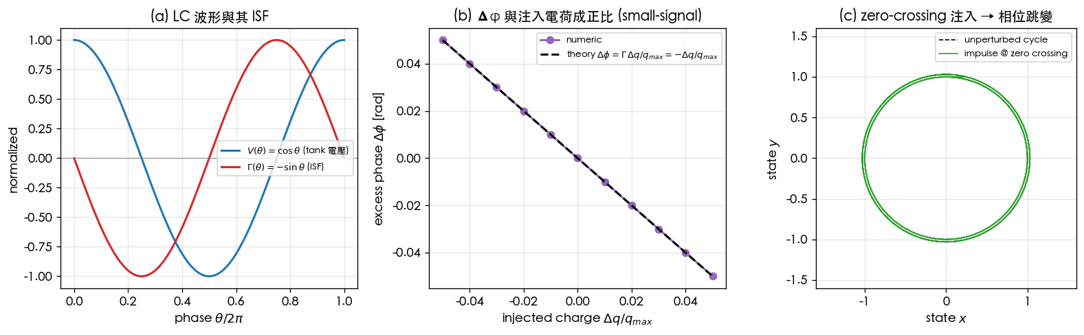
Corresponding formulas $\Gamma_{LC}(\theta)=-\sin\theta$, $\Delta\phi=\Gamma\,\Delta q/q_{max}$; source [P1] Figs. 4, 6, 7(a); script simulations/lab_02_lc_toy_model.py (main), parameters $f_0=1$, $f_s=8000$, $\mu=0.3$, $\Delta q/q_{max}\in[-0.05,0.05]$. This is a pedagogical toy model, not transistor-level.

(2) Measuring $\Gamma$ numerically — seeing is believing: inject a small charge at a sweep of phases, measure the persistent phase offset, and back-solve for the ISF; it lies almost on top of the analytic $-\sin\theta$ (maximum error about 0.001):

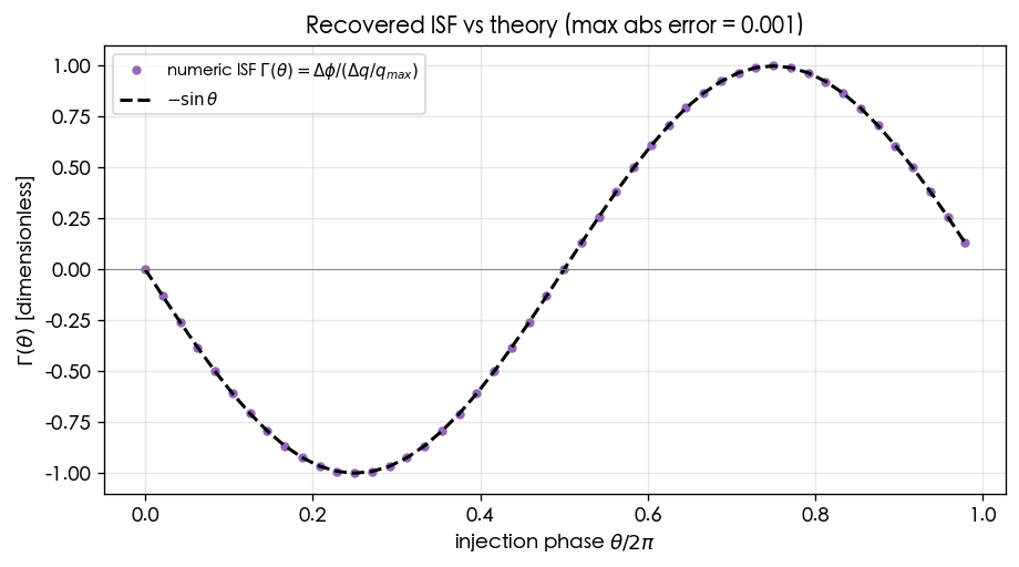
Source: verification of the [P1] ISF definition; script simulations/lab_04_impulse_sweep.py (fig_isf_sweep), $\Delta q/q_{max}=10^{-3}$, 48 phase points. Details in lab_04. Toy model.

Numerical example (building a feel for the numbers)

Example A: $q_{max}=1$ pC, $\Delta q=1$ fC, $\Gamma=0.5$, $f_0=5$ GHz.

Take $\Gamma=0.5$ (note that the ideal-LC $|\Gamma|$ tops out at 1; $\Gamma=0.5$ corresponds to $-\sin\theta=0.5$, i.e. a moderately sensitive phase near $\theta\approx-30^\circ$):

$$\Delta\phi=\frac{\Gamma\,\Delta q}{q_{max}}=\frac{0.5\times(1\times10^{-15}\,\text{C})}{1\times10^{-12}\,\text{C}}=5\times10^{-4}\ \text{rad}\approx0.0286^\circ.$$

Converted to a timing error ($\Delta t=\Delta\phi/(2\pi f_0)$):

$$\Delta t=\frac{5\times10^{-4}\ \text{rad}}{2\pi\times5\times10^{9}\ \text{Hz}}\approx1.59\times10^{-14}\ \text{s}=15.9\ \text{fs}.$$

Dimension check: $[\text{rad}]/[\text{rad/s}]=[\text{s}]$ ✓. Feel for the numbers: 1 fC (about 6240 electrons) at a moderately sensitive phase kicks out only ~16 fs; each kick is tiny, but the noise keeps kicking and the integral accumulates (next page).

from simulations.common.isf_utils import gamma_lc_ideal, impulse_to_phase_step
import numpy as np

# ideal LC ISF: Γ(θ) = -sin(θ)
theta = np.array([0.0, np.pi/2])          # peak, zero crossing
print(gamma_lc_ideal(theta))              # -> [ 0. -1.]  0 at the peak, |Γ|=1 at the zero crossing

dphi = impulse_to_phase_step(delta_q=1e-15, gamma_value=0.5, qmax=1e-12)
print(dphi, "rad")                        # -> 0.0005 rad

(Library: simulations/common/isf_utils.py.)

How the papers' ISF definitions compare

The same $\Gamma$ plays different roles in different papers, but the core object is one and the same:

Source	Symbol / object	Context	Relation to this site's $\Gamma$	Confidence
[P1] Hajimiri–Lee 1998	$\Gamma(\omega_0\tau)$	phase noise (LTV impulse response)	the original source of this site's definition, Eq.(10),(11)	high (equations verified)
[P2] Hajimiri–Limotyrakis–Lee 1999	$\Gamma(\omega_0\tau)$	jitter/phase noise of ring oscillators	the same $\Gamma$; emphasizes the $\Gamma_{rms}\propto N^{-3/2}$ scaling ([P2] Eq.(16), p.794; v7 re-verified: the radical covers only the constant; the text's 4/N^1.5@η=0.75 and App.B Eq.(55) triple-confirm it. An earlier v3 pass misread this as N^-0.75)	high (statement and scaling both verified)
[P3] Hong–Hajimiri 2019 Part I	$\Gamma(\theta+\phi)$	injection locking/pulling (generalized Adler)	the same $\Gamma$, moved to the injection context: $\frac{d\phi}{dt}=\Delta\omega-\frac{1}{q_{max}}\langle\Gamma(\theta+\phi)\,i_{inj}(\theta)\rangle$ ([P3] Eq.(30), p.2113; this site's $\Gamma$ adopts the sign convention opposite to [P3], hence the $-$ in front of the averaged term — numerically equivalent)	high (checked against the original PDF)
[P4] Hong–Hajimiri 2019 Part II	$\Lambda(\phi)$ (APF)	amplitude modulation (amplitude domain)	the amplitude version: projects the impulse onto the radial rather than the tangential direction; units $\text{A}^{-1}$; in the ideal LC the ISF and APF are in quadrature ([P4] Eq.(26), p.2128)	✓ (APF=[P4] Eq.(19), Fig. 5, p.2126, verified)
[P5] Hajimiri–Heald 1998	—	sense amplifier	unrelated to the ISF (a sense-amplifier paper, honestly flagged as mislabeled)	high (clearly off-topic)

Notation trap: [P3] writes $\Gamma(\theta+\phi)$, taking "the injection waveform phase $\theta$" plus "the oscillator's own excess phase $\phi$" as the argument — in essence it is still the same $\Gamma$, only with the argument recast as a relative phase. The APF $\Lambda$ of [P4] is the amplitude sensitivity, complementary to $\Gamma$ (the phase sensitivity); in the ideal LC the two are orthogonal (one $\propto\sin$, the other $\propto\cos$). See paper_004_injection_locking_part2.

Verified: the [P3] generalized Adler equations (Eq.30/33, p.2113–2114) and the [P4] APF (Eq.25/26, p.2128) have been checked against the original PDFs; see the paper_003 / paper_004 deep-dives.

Where it applies, where it fails

Condition	When it holds	What happens when it fails
Small signal $\Delta q\ll q_{max}$	tangential projection is linear; $\Gamma$ independent of $\Delta q$	large injection → nonlinearity, AM–PM, $\Gamma$ itself is altered
Stable limit cycle (amplitude perturbations decay)	only the phase needs tracking	with no stable cycle or strong AM–PM, the phase-only model breaks down
Large-signal periodic steady-state waveform is known	the shape of $\Gamma$ can be determined	unknown waveform → unknown projection direction; extract by transient/adjoint
Pulse far narrower than the period $T$	can be treated as instantaneous injection	wide pulses require the integral form, Eq.(11) (see next page)

Worked examples

Format per spec §10.4: problem → step-by-step substitution (with units) → result → dimension check → one-line Python verification.

Example 1: $\Gamma=-\sin$ at $\theta=0,\pi/4,\pi/2$ and the resulting $\Delta\phi$

Problem: the ideal LC has $\Gamma(\theta)=-\sin\theta$. Inject the same packet of charge at three phases — $\theta=0$ (peak), $\theta=\pi/4$ (halfway), $\theta=\pi/2$ (zero crossing) — with the injected-charge ratio fixed at $\Delta q/q_{max}=10^{-3}$. Find $\Gamma$ and the phase step $\Delta\phi=\Gamma\cdot\Delta q/q_{max}$ at each point.

Step-by-step substitution: compute $\Gamma$ first, then multiply by $\Delta q/q_{max}=10^{-3}$.

$$\begin{aligned} \theta=0:\quad &\Gamma=-\sin0=0, &\Delta\phi&=0\times10^{-3}=0\ \text{rad}.\\ \theta=\tfrac{\pi}{4}:\quad &\Gamma=-\sin\tfrac{\pi}{4}=-\tfrac{1}{\sqrt2}\approx-0.7071, &\Delta\phi&=-0.7071\times10^{-3}=-7.07\times10^{-4}\ \text{rad}.\\ \theta=\tfrac{\pi}{2}:\quad &\Gamma=-\sin\tfrac{\pi}{2}=-1, &\Delta\phi&=-1\times10^{-3}=-1.0\times10^{-3}\ \text{rad}. \end{aligned}$$

Result: the same packet of charge barely moves the phase at the peak ($\Delta\phi=0$), delivers the maximum phase step at the zero crossing ($|\Delta\phi|=1$ mrad), and lands in between at the halfway point ($0.707$ mrad). This is the core LTV phenomenon: the effect is decided by when you strike.

Dimension check: $\Gamma$ dimensionless, $\Delta q/q_{max}$ dimensionless → $\Delta\phi$ dimensionless (rad) ✓. The minus sign means the phase is pushed backward (it lags); the order of magnitude is set by $\Delta q/q_{max}$, the same order as Example A's $5\times10^{-4}$ rad (Example A uses $\Gamma=0.5$).

import numpy as np
from simulations.common.isf_utils import gamma_lc_ideal, impulse_to_phase_step
theta = np.array([0.0, np.pi/4, np.pi/2])
g = gamma_lc_ideal(theta)                       # -> [ 0.    -0.7071 -1.    ]
dphi = impulse_to_phase_step(delta_q=1e-3, gamma_value=g, qmax=1.0)  # Δq/qmax = 1e-3
print(g)                                        # ISF values
print(dphi)                                     # -> [ 0.  -7.07e-04  -1.0e-03 ] rad

Example 2: converting the zero-crossing injection into a timing error at 5 GHz

Problem: continuing Example 1 at $\theta=\pi/2$ ($|\Delta\phi|=1$ mrad), convert to a timing error $\Delta t=\Delta\phi/(2\pi f_0)$ at $f_0=5$ GHz.

Step-by-step substitution:

$$\Delta t=\frac{1\times10^{-3}\ \text{rad}}{2\pi\times5\times10^{9}\ \text{Hz}}=\frac{10^{-3}}{3.1416\times10^{10}}\ \text{s}\approx3.18\times10^{-14}\ \text{s}=31.8\ \text{fs}.$$

Result: a single injection at the most sensitive phase with $\Delta q/q_{max}=10^{-3}$ produces about 31.8 fs of timing error at 5 GHz (echoing the "1 mrad ≈ 32 fs" anchor in numerical_feeling).

Dimension check: $[\text{rad}]/[\text{rad/s}]=[\text{s}]$ ✓ ($2\pi f_0$ is in rad/s).

from simulations.common.noise_utils import phase_to_time_error
print(phase_to_time_error(1e-3, 5e9)*1e15, "fs")   # -> 31.83 fs

(Libraries: simulations/common/isf_utils.py, simulations/common/noise_utils.py.)

Key takeaways

• $\Gamma(\omega_0\tau)$ = the sensitivity weight answering "inject one unit of charge at waveform phase $\omega_0\tau$ — how much becomes permanent phase?"
• The derivation chain: impulse → charge $\Delta q$ → voltage step $\Delta V$ → state displacement → projection onto the tangent (the phase direction) → permanent phase $\Delta\phi$.
• $\Gamma$ is dimensionless, $2\pi$-periodic, not the noise itself, set by the large-signal periodic operating point, and there is one per node / per noise source.
• Ideal LC: $\Gamma(\theta)=-\sin\theta$ — peak injection gives $\Gamma=0$ (amplitude only), zero crossing gives $|\Gamma|=1$ (maximum phase) — that is LTV.
• Across the papers: [P1][P2] use $\Gamma$ for phase noise; [P3] applies the same $\Gamma$ to injection; [P4]'s APF $\Lambda$ is the amplitude counterpart; [P5] is unrelated to the ISF.
• Sources: [P1] Eqs.(10),(11), p.182; verification figures in lab_02 / lab_04.

Further reading

• The operational step-by-step derivation: impulse_to_phase_shift
• Superposition over arbitrary noise (the convolution form): convolution_derivation
• The Fourier series of $\Gamma$ and frequency translation: fourier_series_of_isf
• Cyclostationary noise and the effective ISF (incl. PPV/adjoint external literature): effective_isf
• Phase-vs-amplitude geometry: phase_vs_amplitude_noise, oscillator_phase