β: This English translation is in beta — the Traditional-Chinese original is the authoritative version.
Numerical Feeling
However beautiful the theory, without numbers there is no feel. This page uses three small
examples to turn the conversions among phase, time, dBc/Hz, and jitter
into reflexes. Each example comes with a Python check; the full library lives in
simulations/common/.
Formula sources: the phase/time/jitter conversions and the 1/f² integral are all standard results, consistent with [P1] A. Hajimiri and T. H. Lee, "A General Theory of Phase Noise in Electrical Oscillators," IEEE JSSC, 33(2), 1998 (especially Eq.(21)); step-by-step derivations in impulse_to_phase_shift and psd_phase_noise_jitter.
Why drill the numbers first: an analog designer's ability to estimate orders of magnitude at the whiteboard matters more than memorizing formulas. Given " dBc/Hz @ 1 MHz, 5 GHz," you should be able to estimate "a few hundred fs of jitter" within 30 seconds.
Example 1: phase → time
Given GHz and mrad, find the timing error.
- Dimension check: ✓ ( is in rad/s).
- Feel: at 5 GHz, "1 mrad ≈ 32 fs." The period is 200 ps, so 1 mrad is about of a period.
from simulations.common.noise_utils import phase_to_time_error
print(phase_to_time_error(1e-3, 5e9) * 1e15, "fs")   # -> 31.83 fs
Example 2: injected charge → phase step → time
Given pC, fC, , find the phase step and the timing error (at 5 GHz).
Phase step:
Timing error ( GHz):
- Feel: 1 fC ≈ 6240 electrons; even at the most sensitive phase it only kicks out ~16 fs. Each kick is tiny, but noise keeps kicking and the phase integrator accumulates it (see convolution_derivation).
- Full derivation in impulse_to_phase_shift (Example A).
from simulations.common.isf_utils import impulse_to_phase_step
from simulations.common.noise_utils import phase_to_time_error
dphi = impulse_to_phase_step(1e-15, 0.5, 1e-12)
print(dphi, "rad ->", phase_to_time_error(dphi, 5e9)*1e15, "fs")  # 0.0005 rad -> 15.92 fs
Example 3: phase noise plot → rms jitter (you must be able to integrate)
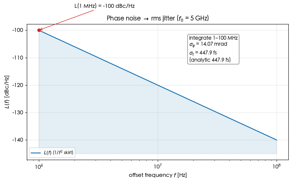
Given dBc/Hz, assuming a 1/f² slope, integrating from 1 MHz to 100 MHz, GHz, estimate the rms jitter.
Step 1: convert dBc/Hz to linear and recover the phase PSD. Under the single-tone small-angle approximation , so . At 1 MHz: dBc/Hz , rad²/Hz.
Step 2: write down the 1/f² shape. Anchored at MHz:
Step 3: integrate to get the phase variance.
Step 4: convert to rms jitter.
- Feel: the integral is dominated by the lower limit (the term is largest) — so "where you start integrating" is critical for 1/f².
- Reference point: if this part were dBc/Hz @ 1 MHz (10× better in power, × in voltage), the jitter shrinks to roughly ~45 fs.
- This is exactly the figure of lab_08; the numerical integration matches the analytic expression exactly.
import numpy as np
from simulations.common.noise_utils import leeson_one_over_f2, integrate_rms_jitter

f  = np.logspace(6, 8, 4000)                 # 1 MHz -> 100 MHz
L  = leeson_one_over_f2(f, L_ref_dbc=-100, f_ref=1e6)   # 1/f^2 skirt
sigma_t, sigma_phi = integrate_rms_jitter(f, L, f0=5e9, fmin=1e6, fmax=100e6)
print(sigma_phi*1e3, "mrad ;", sigma_t*1e15, "fs")   # -> 14.07 mrad ; 447.9 fs
Full script: simulations/lab_08_jitter_integration.py.
Parameter and unit quick reference
| Quantity | Symbol | Unit | Conversion |
|---|---|---|---|
| Phase error | rad | rad | |
| Timing error | s | ||
| phase PSD | rad²/Hz | ||
| SSB phase noise | dBc/Hz | (→ dB) | |
| Charge | C | 1 fC C |
Key takeaways
- 5 GHz conversion anchors: 1 mrad ≈ 32 fs; 1 rad ≈ 31.8 ps.
- dBc/Hz → linear → linear → integrate → square root → = rms jitter.
- 1/f² jitter is dominated by the lower integration limit.
- All the numbers in these three examples can be checked in one line with the built-in functions in
simulations/common/.