Lab 01 — Sinusoidal Oscillator and the Phase/Amplitude Geometry of the Limit Cycle

β: This English translation is in beta — the Traditional-Chinese original is the authoritative version.

This is the first lab of the entire ISF (Impulse Sensitivity Function — the oscillator's "phase-sensitivity" weight toward noise) story. We deliberately touch no constants in any formula yet; with a single 2-D picture we build a geometric intuition that will stay with you for life: the oscillator's state circles a closed trajectory (the limit cycle); when a perturbation pushes the state point away, the part along the cycle (tangential) becomes phase and the part off the cycle (radial) becomes amplitude; and phase has no restoring force while amplitude does — this is the root of "why phase noise accumulates permanently".

Physical intuition (conclusion first): picture the oscillation as a bead circling a track at constant speed. Push it from the side (tangentially) → its position along the track (the phase) is permanently displaced; no force whatsoever pushes it back to its original schedule. Push it inward from the outside (radially) → the track radius (the amplitude) changes, but the oscillator's AGC / device nonlinearity slowly pulls the radius back to steady state. So only the tangential part becomes a permanent phase error. The same impulse, injected at different phases of the waveform, splits between tangential and radial in different proportions — this is exactly what the ISF $\Gamma(\omega_0\tau)$ describes.

1. Learning goals

• See the limit cycle in the 2-D state space, and distinguish the geometric directions of the two perturbations: phase (tangential) and amplitude (radial).
• Understand that amplitude perturbations are pulled back to the limit cycle by a restoring mechanism, while phase perturbations remain permanently.
• See why a current impulse of the same size changes almost only the amplitude when injected at the peak ($\Gamma\approx0$) and almost only the phase at the zero crossing ($|\Gamma|$ maximal) — the most direct evidence that the ISF is time-variant (LTV) rather than time-invariant (LTI).
• Lay the geometric groundwork for $\Gamma(\theta)=-\sin\theta$ in lab_02 and the derivation in impulse_to_phase_shift.

2. Mathematical model

We use a normalized (dimensionless) 2-D oscillator state model. The state is $z=(x,y)$, where you may think of $x$ as the capacitor voltage and $y$ as (proportional to) the inductor current:

$$\begin{aligned} \frac{dx}{dt}&=-\omega_0\,y+\mu\,(1-r^2)\,x,\\ \frac{dy}{dt}&=\;\;\omega_0\,x+\mu\,(1-r^2)\,y,\qquad r^2=x^2+y^2. \end{aligned}$$

• The first term, the $\pm\omega_0$ coupling: pure rotation. With $\mu=0$ this is the ideal lossless LC: the state circles the unit circle at constant angular velocity $\omega_0$, with the amplitude marginally stable (neither growing nor decaying), corresponding to $V(t)=\cos\omega_0 t$.
• The second term, $\mu(1-r^2)z$: a Van der Pol-style amplitude restoration. For $r>1$ (pushed outside the circle) it pulls inward; for $r<1$ (pushed inside) it pushes outward — dragging the trajectory back to the $r=1$ limit cycle. It models the AGC / device nonlinearity every real oscillator must have (without it, the amplitude would diverge or decay).
• Dimension check: the equations are normalized — $x,y,r$ are all dimensionless, $\omega_0,\mu$ carry rad/s, and both sides are "dimensionless ÷ seconds" ✓.

How a perturbation enters: a current impulse injected into the capacitor node deposits charge $\Delta q=\int i\,dt$, producing an instantaneous voltage step $\Delta V=\Delta q/C_{node}$ ([P1] Eq.(9), p.182):

$$\Delta V=\frac{\Delta q}{C_{node}}.$$

In normalized units ($A=1$, $q_{max}=C_{node}\cdot A=C_{node}$), this is a step $\Delta x=\Delta q/q_{max}$ added to the $x$ state. Note that it moves only the capacitor voltage $x$, not the inductor current $y$ (an inductor current cannot change instantaneously), so in the state space it is a horizontal jump along the $x$ axis — Step 2 of impulse_to_phase_shift covers this in more detail.

Toy-model statement: this is a pedagogical toy model, not transistor-level. It faithfully reproduces the mechanisms — the phase/amplitude decomposition and the absence of a phase restoring force — but it produces no noise numbers of any real circuit.

3. Block diagram

4. Core Python code

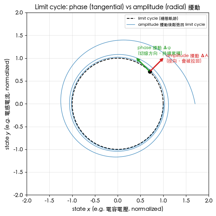
The following is excerpted from the actual script (checked against simulations/lab_01_sinusoidal_oscillator.py). fig_limit_cycle starts integrating from a point off the cycle, $(x_0,y_0)=(1.7,0)$, so you can watch the trajectory relax back to the limit cycle; two arrows then mark the tangential (phase) and radial (amplitude) directions:

from oscillator_models import simulate_lc, sinusoidal_oscillator

def fig_limit_cycle():
    f0 = 1.0          # normalized
    fs = 4000.0
    # start from an off-cycle point: the trajectory relaxes back to the unit-circle limit cycle (mu=0.6 provides amplitude restoration)
    t, x, y = simulate_lc(f0, t_end=3.0, fs=fs, mu=0.6, x0=1.7, y0=0.0)

    # operating point chosen at theta = pi/4
    p = np.array([np.cos(np.pi / 4), np.sin(np.pi / 4)])
    tang = np.array([-p[1], p[0]]) * 0.45   # tangential (phase) direction: perpendicular to the radius
    rad  = p * 0.45                          # radial (amplitude) direction: along the radius
    # tang part -> permanent phase Δφ ; rad part -> amplitude ΔA, pulled back

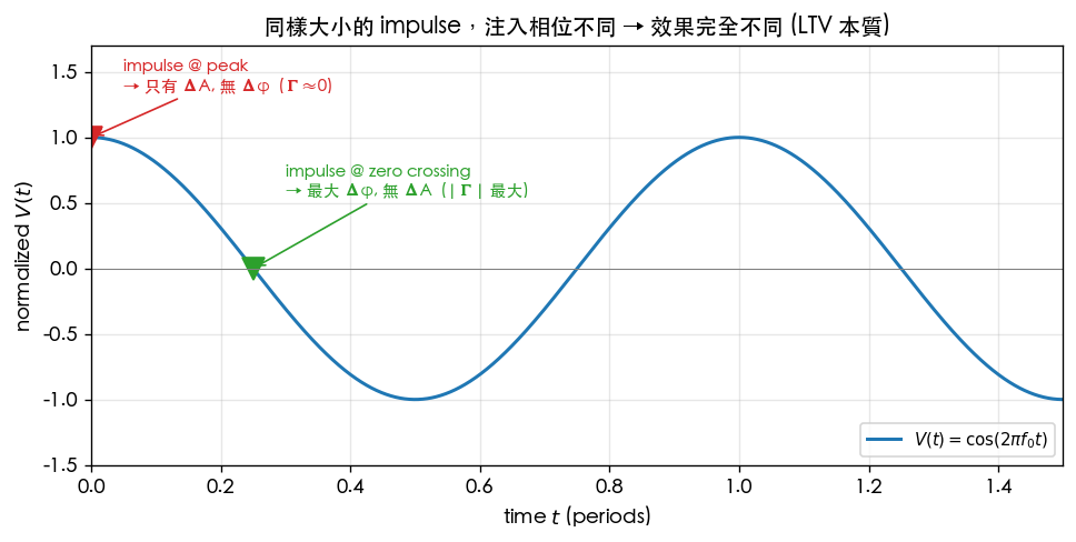
The second figure marks equal-size impulses at the peak ($\theta=0$) and at the zero crossing ($\theta=\pi/2$, i.e. $t=0.25T$), highlighting that "the injection phase determines the effect":

def fig_impulse_markers():
    f0, fs = 1.0, 4000.0
    t = np.arange(int(2.0 * fs)) / fs
    v = sinusoidal_oscillator(t, f0, amp=1.0)   # V(t)=cos(2*pi*f0*t)

    t_peak = 0.0          # peak theta=0  -> amplitude only (Gamma ~ 0)
    t_zc   = 0.25 / f0    # zero crossing theta=pi/2 -> phase only (|Gamma| max)

The underlying state integration (RK4) and impulse injection live inside simulate_lc(); injection is xi += impulse_dx, i.e. adding a step of $\Delta q/q_{max}$ to the $x$ state.

5. Full script path

simulations/lab_01_sinusoidal_oscillator.py (depends on simulate_lc and sinusoidal_oscillator from simulations/common/oscillator_models.py, and savefig from simulations/common/plot_utils.py.)

To run: python scripts/run_all_sims.py (generates all site figures into static/figures/), or standalone: python simulations/lab_01_sinusoidal_oscillator.py.

6. Parameter table

Parameter	Code variable	Value	Meaning
Oscillation frequency	f0	1.0 (normalized)	this lab looks only at shape, so dimensionless frequency
Sampling rate	fs	4000	4000 points per period, smooth enough
Amplitude-restoring strength	mu	0.6 (limit-cycle figure) / 1.0	Van der Pol coefficient; larger pulls back to the cycle faster
Initial state	x0, y0	(1.7, 0.0)	deliberately off the cycle, to show relaxation back to the limit cycle
Peak injection phase	$\theta$	0	$\Gamma\approx0$: amplitude change only
Zero-crossing injection phase	$\theta$	$\pi/2$ ($t=0.25T$)	$\vert \Gamma\vert$ maximal: phase change only

7. Units table

Quantity	Symbol	Unit	Note
Time	$t$	periods (normalized)	plot x-axes count in periods
State $x$	$x$	normalized (≈ capacitor voltage)	dimensionless
State $y$	$y$	normalized (≈ inductor current)	dimensionless
Angular frequency	$\omega_0=2\pi f_0$	rad/s	$=2\pi$ when normalized
Phase perturbation	$\Delta\phi$	rad	tangential component; permanent
Amplitude perturbation	$\Delta A$	normalized	radial component; decays
ISF	$\Gamma(\omega_0\tau)$	dimensionless	tangential/radial split ratio

8. Simulation figures

(Figure 1) Phase vs amplitude perturbations on the limit cycle

(Figure 2) Same-size impulse at different injection phases → completely different effects

9. How to read the figures

Figure 1 (state space):

• The black dashed unit circle is the steady-state limit cycle; the solid blue curve is the trajectory starting from $(1.7,0)$, pulled back to the unit circle turn after turn by the $\mu(1-r^2)z$ term — seeing is believing for "amplitude perturbations get restored".
• The black dot is the operating point $\theta=\pi/4$. The green arrow (tangential) is the phase direction: moving along the cycle is moving the bead forward/backward on the track, and no force pushes it back, so this part accumulates permanently.
• The red arrow (radial) is the amplitude direction: pushing the point away from or toward the center gets pulled back by the restoring mechanism, leaving no trace.
• Key mental model: any perturbation vector decomposes into these two orthogonal components; only the part projected onto the green tangential direction becomes permanent phase error.

Figure 2 (waveform):

• The blue curve is $V(t)=\cos(2\pi f_0 t)$. The red triangle sits at the peak: the waveform slope there is 0, so the horizontal voltage jump is almost purely radial (amplitude change), with tangential component $\approx0$, hence $\Gamma\approx0$.
• The green triangle sits at the zero crossing: the waveform slope there is maximal, so the horizontal voltage jump is almost purely tangential (phase change), hence $|\Gamma|$ is maximal.
• Connect the two points: the same $\Delta q$ at different injection times $\tau$ → completely different $\Delta\phi$. The system's response to an impulse depends on the absolute injection phase — the defining signature of LTV (compare lti_vs_ltv).

10. Corresponding paper equations/figures

• Conceptual source: [P1] Fig. 4, p.182 — Hajimiri–Lee use the state-space limit cycles of LC and ring oscillators to demonstrate "impulse at the peak (amplitude change) vs at the zero crossing (phase change)". The two figures in this lab are redrawn conceptual toy figures (redrawn conceptual — not transistor-level, not point-by-point copies of the paper's figures).
• Charge → voltage step: [P1] Eq.(9), p.182, $\Delta V=\Delta q/C_{node}$.
• ISF and impulse response (used in the next step): [P1] Eq.(10), p.182:

$$h_\phi(t,\tau)=\frac{\Gamma(\omega_0\tau)}{q_{max}}\,u(t-\tau).$$

where the unit step $u(t-\tau)$ is exactly the mathematical statement of Figure 1's "phase perturbations remain permanently".

• Next: the ideal LC's $\Gamma(\theta)=-\sin\theta$ (maximal at the zero crossings, zero at the peaks — consistent with Figure 2) is derived in lab_02 and isf_definition.

11. Limitations and approximations

• This is a pedagogical toy model, not transistor-level. $\mu(1-r^2)z$ is only the simplest possible way to write "there is amplitude restoring"; it does not represent the restoring dynamics of any real device — real amplitude-restoring time constants and AM–PM conversion require transistor-level / Floquet analysis.
• Small-signal assumption: projecting a perturbation into "tangential + radial" is a linearization, requiring $\Delta q\ll q_{max}$. A large injection nonlinearly alters the ISF itself (see the linearity verification in lab_02).
• Narrow-pulse assumption: treating the impulse as an instantaneous voltage jump requires the pulse width $\ll T$; wide pulses must go back to the integral form of Eq.(11).
• This lab deliberately gives no absolute-unit numbers (normalized $f_0=1$) — it teaches the geometry and the sign directions. The canonical numbers with real units ($q_{max}=1$ pC, $\Delta q=1$ fC, $f_0=5$ GHz, $\Delta\phi=5\times10^{-4}$ rad, $\Delta t=15.9$ fs) are in Example A of impulse_to_phase_shift and in numerical_feeling.

Key takeaways

• The oscillator state circles the limit cycle; a perturbation decomposes into tangential (phase, permanent) and radial (amplitude, pulled back).
• Phase has no restoring force — the physical root of phase noise accumulating without bound (random walk).
• Same-size impulse: at the peak → amplitude change ($\Gamma\approx0$); at the zero crossing → phase change ($|\Gamma|$ maximal).
• "The effect depends on the injection phase" = the essence of LTV, and the reason the ISF exists.
• Source: [P1] Fig. 4 and Eq.(9),(10), p.182.