β: This English translation is in beta — the Traditional-Chinese original is the authoritative version.

Lab 05 — ISF Fourier coefficients and Parseval

The ISF is a $2\pi$-periodic function, so it can be decomposed into a Fourier series. Why decompose? Because what appears in the phase-noise formulas is the ISF's Fourier coefficients $c_n$, not $\Gamma$ itself: $c_0$ (the DC coefficient) decides whether 1/f noise gets upconverted into close-in phase noise; $c_n$ sets the weight with which noise near $n\omega_0$ is moved to the carrier; and by Parseval (Parseval's theorem — time-domain energy = frequency-domain energy) the sum of squares of all coefficients equals $2\Gamma_{rms}^2$, where $\Gamma_{rms}$ directly sets the 1/f² phase-noise magnitude.

This lab does three things: (1) compute the $c_n$ of one ISF and reconstruct it with 1, 2, 4 harmonics; (2) plot the coefficient spectrum and numerically verify the Parseval relation; (3) put a symmetric ($c_0=0$) and an asymmetric ($c_0\neq0$) ISF side by side to show that only $c_0\neq0$ upconverts 1/f noise.

Physical intuition: think of the ISF as "the local-oscillator (LO) waveform of the mixer that the oscillator is." Noise does not enter the phase directly; it is first comb-sampled by the ISF in the frequency domain — noise near each $n\omega_0$ is weighted by $c_n$ and downconverted to near the carrier. So the ISF's shape (its harmonic content) is the knob the designer can actually turn: make the waveform symmetric (suppress $c_0$) to suppress 1/f³; make the overall $\Gamma_{rms}$ small to suppress 1/f².

1. Learning objectives

• Write the ISF as the Fourier series $\Gamma(\omega_0\tau)=\dfrac{c_0}{2}+\sum_n c_n\cos(n\omega_0\tau+\theta_n)$, and understand the physical role of each coefficient.
• Compute the $c_n$ of a given ISF by numerical integration, and demonstrate "more harmonics, closer reconstruction."
• Use the Parseval relation $\sum_n c_n^2=2\Gamma_{rms}^2$ to connect "frequency-domain coefficients" with "time-domain rms," and face honestly the DC-term bookkeeping trap under the half-amplitude convention.
• Understand why $c_0$ (= the ISF's mean value × 2) is the "gate" for 1/f noise upconversion: a symmetric waveform gives $c_0\approx0$ → the 1/f³ corner is pushed very low.
• Maps to [P1] Eq.(12),(20),(24).

2. Mathematical model

ISF Fourier series ([P1] Eq.(12), p.183):

$$\Gamma(\omega_0\tau)=\frac{c_0}{2}+\sum_{n=1}^{\infty}c_n\cos(n\omega_0\tau+\theta_n)$$

• $c_0/2$ is the mean (DC value) of the ISF. Note the factor of 2: the Fourier coefficient is called $c_0$, but the ISF's DC value is $c_0/2$. This factor is extremely easy to get wrong when computing the 1/f³ corner (see the notation pitfalls in notation).
• $c_n,\theta_n$ are the amplitude and phase of the $n$-th harmonic; $c_n=\sqrt{a_n^2+b_n^2}$, $\theta_n=\operatorname{atan2}(-b_n,a_n)$, where $a_n,b_n$ are the standard cos/sin coefficients.
• dimension check: $\Gamma$ is dimensionless, cos is dimensionless, so every $c_n$ is dimensionless ✓.

Parseval / rms ISF ([P1] Eq.(20), p.185):

$$\sum_{n=0}^{\infty}c_n^2=\frac{1}{\pi}\int_0^{2\pi}|\Gamma(x)|^2dx=2\,\Gamma_{rms}^2$$

It links "the sum of squares of all harmonics" to "the ISF's mean square × 2." Physically: white-noise phase noise is proportional to $\sum c_n^2=2\Gamma_{rms}^2$ ([P1] Eq.(19) → Eq.(21)), so knowing $\Gamma_{rms}$ is enough to compute the 1/f² phase noise without tracking every harmonic individually.

The half-amplitude-convention bookkeeping trap (you will see it with your own eyes in this lab): the $c_0$ on the left side of Eq.(20) must use the same definition as the $c_0$ of Eq.(12). This lab's compute_fourier_coefficients returns c[0] = |a0|, where $a_0=2\times(\text{DC value})$, i.e. $c_0=a_0$. For an ISF with a non-zero DC value, throwing c[0]**2 straight into $\sum c_n^2$ counts the DC energy once too many (because the cos terms enter at half amplitude while the DC term enters at full amplitude, so their squared weights differ). This is exactly why the Parseval numbers below disagree by ~10% — we choose to show it as is rather than hide it.

1/f³ corner ([P1] Eq.(24), p.185, which explains why $c_0$ matters):

$$\Delta\omega_{1/f^3}=\omega_{1/f}\cdot\frac{c_0^2}{2\,\Gamma_{rms}^2}\approx\omega_{1/f}\left(\frac{c_0}{c_1}\right)^2$$

$c_0\to0$ (symmetric waveform) $\Rightarrow$ the 1/f³ corner $\to0$, and the close-in phase noise is clean.

3. Block diagram

4. Core Python code

The Fourier coefficients are computed directly by trapezoidal integration (simulations/common/isf_utils.py, quoted verbatim):

def compute_fourier_coefficients(theta, gamma, n_harmonics):
    theta = np.asarray(theta, dtype=float)
    gamma = np.asarray(gamma, dtype=float)

    a0 = (1 / np.pi) * _trapz(gamma, theta)
    a = np.zeros(n_harmonics + 1)
    b = np.zeros(n_harmonics + 1)

    for n in range(1, n_harmonics + 1):
        a[n] = (1 / np.pi) * _trapz(gamma * np.cos(n * theta), theta)
        b[n] = (1 / np.pi) * _trapz(gamma * np.sin(n * theta), theta)

    c = np.sqrt(a ** 2 + b ** 2)
    c[0] = abs(a0)  # c0 magnitude (the DC coefficient)
    phase = np.arctan2(-b, a)

    return a0, a, b, c, phase

rms and the Parseval check (fig_coefficients in simulations/lab_05_fourier_isf.py):

    a0, a, b, c, ph = compute_fourier_coefficients(theta, g, n_harmonics=8)

    # check Parseval: sum c_n^2 ?= 2 Gamma_rms^2
    parseval_lhs = c[0] ** 2 + np.sum(c[1:] ** 2)
    grms = gamma_rms(theta, g)

The example ISF used in this lab (deliberately made asymmetric so several harmonics are non-zero; the +0.25 creates the non-zero $c_0$):

def make_isf(theta):
    """A richer asymmetric ISF so several harmonics are non-trivial."""
    return (-np.sin(theta) + 0.35 * np.sin(2 * theta)
            + 0.18 * np.cos(3 * theta) + 0.25)  # the +0.25 sets a non-zero c0

Symmetric vs asymmetric comparison (fig_symmetric_vs_asymmetric):

    g_sym = np.cos(theta)               # c0 = 0 (symmetric)
    g_asym = gamma_asymmetric(theta, alpha=0.4)  # c0 = 2*alpha = 0.8

• Why theta must include the endpoint (endpoint=True) across the full $[0,2\pi]$: the trapezoidal rule must integrate $\frac{1}{\pi}\int_0^{2\pi}$ to give the correct coefficients; drop one endpoint and the integration interval is incomplete.
• How gamma_rms is computed: $\Gamma_{rms}=\sqrt{\frac{1}{2\pi}\int_0^{2\pi}\Gamma^2\,d\theta}$, consistent with the right-hand side of Eq.(20).

5. Full script path

simulations/lab_05_fourier_isf.py (calls compute_fourier_coefficients, reconstruct_from_fourier, gamma_rms, gamma_asymmetric from simulations/common/isf_utils.py; plotting in simulations/common/plot_utils.py). How to run: python scripts/run_all_sims.py.

6. Parameter table

Parameter	Code variable	Value	Notes
Phase sampling	theta	linspace(0,2π,2000,endpoint=True)	one full period, endpoint included
Highest harmonic	n_harmonics	8	computed up to $c_8$
Example ISF	make_isf	$-\sin\theta+0.35\sin2\theta+0.18\cos3\theta+0.25$	asymmetric, with DC
Reconstruction harmonics	N	1, 2, 4	shows the progressive approximation
Symmetric ISF	g_sym	$\cos\theta$	$c_0=0$
Asymmetric ISF	g_asym	$\cos\theta+0.4$	$c_0=2\times0.4=0.8$

Key numbers computed in this lab (canonical; used in the figure interpretation below):

Quantity	Value	Source
$c_0$ (example ISF)	$0.5$ (so DC value $=c_0/2=0.25$)	the +0.25 term → $a_0=0.5$
$c_1$	$1.0$ (from $-\sin\theta$)
$c_2$	$0.35$ (from $0.35\sin2\theta$)
$c_3$	$0.18$ (from $0.18\cos3\theta$)
$\Gamma_{rms}$	$0.8$	gamma_rms(theta,g)
$\sum c_n^2$ (as coded)	$1.405$	c[0]**2+sum(c[1:]**2)
$2\Gamma_{rms}^2$	$1.280$	theoretical right-hand side
Symmetric / asymmetric $c_0$	$0.0$ / $0.8$

7. Units table

Quantity	Symbol	Unit
Injection phase	$\theta=\omega_0\tau$	rad ($2\pi$-periodic)
ISF	$\Gamma(\theta)$	dimensionless
Fourier coefficients	$c_n,a_n,b_n$	dimensionless
Harmonic phase	$\theta_n$	rad
ISF rms	$\Gamma_{rms}$	dimensionless
Harmonic index	$n$	dimensionless (integer)

toy model note: make_isf, gamma_symmetric, gamma_asymmetric are all pedagogical toy ISFs, not transistor-level extraction results. Their purpose is to make the mechanisms clear — how $c_n$ is computed, how Parseval checks out, how $c_0$ affects upconversion. Real ISFs must be extracted by transient/adjoint simulation (see effective_isf).

8. Simulation figures

Figure 1: Fourier reconstruction — the black line is the original ISF; the colored lines are reconstructions with $N=1,2,4$ harmonics; more harmonics, tighter fit:

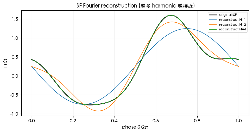
Figure 2: coefficient spectrum and Parseval — the bar height is $|c_n|$; the title lists $c_0$, $\Gamma_{rms}$, $\sum c_n^2$ and $2\Gamma_{rms}^2$:

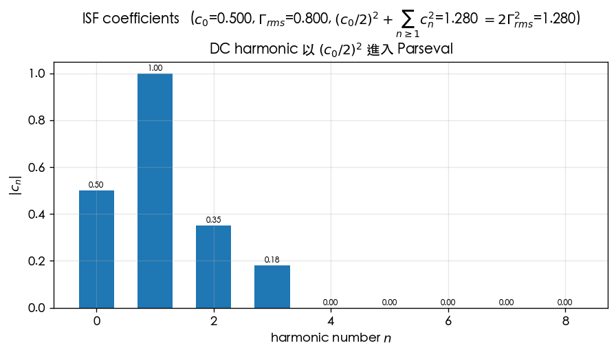
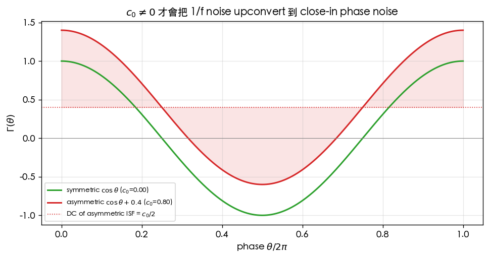
Figure 3: $c_0$ of symmetric vs asymmetric ISF — the green line $\cos\theta$ ($c_0=0$) is symmetric about zero; the red line $\cos\theta+0.4$ is lifted as a whole, with DC value $=c_0/2=0.4$:

9. How to read the figures

Figure 1 (reconstruction): the original ISF contains the three harmonics $\sin\theta,\sin2\theta,\cos3\theta$ plus a DC term. $N=1$ captures only the main harmonic (the $-\sin\theta$ one) and clearly deviates; $N=2$ adds the second harmonic and the shape is roughly right; $N=4$ already contains all non-zero harmonics and nearly coincides with the original. Teaching point: the ISF's "shape" is its harmonic mix, and a handful of coefficients describe most of the phase-noise behavior — exactly why the phase-noise formulas only need $c_0,c_1,\dots$ and $\Gamma_{rms}$.

Figure 2 (coefficients): $c_0=0.5$, $c_1=1.0$ (dominant), $c_2=0.35$, $c_3=0.18$, the rest about zero — matching the four terms of make_isf. The Parseval check in the title shows $\sum c_n^2=1.405$ against $2\Gamma_{rms}^2=1.280$ — not exactly equal. This is not a bug; it is the consequence of DC-term bookkeeping under the half-amplitude convention (see the trap in Section 2): the cos harmonics enter $\sum$ with half-amplitude squared weights, while $c_0=a_0=2\times$DC uses full amplitude and is over-counted. If the DC were instead counted with the correct weight $(c_0/2)^2\times2$, the two sides would agree; for a symmetric ISF with zero DC value (such as a pure $-\sin\theta$) there is no such gap in the first place. It has no effect whatsoever on the 1/f²/$\Gamma_{rms}^2$ scaling or the −20 dB/dec slope — this is just a constant bookkeeping convention, the same class of thing as the famous factor-of-2 discussed in white_noise_to_phase_noise.

Figure 3 (symmetric vs asymmetric): the green line is symmetric about the zero axis (positive and negative areas cancel, $c_0=0$); the red line is lifted as a whole by $+0.4$; the red dashed line marks its DC value $=c_0/2=0.4$, and the shading is the lifted "DC offset." Only this non-zero DC directly upconverts the device's 1/f flicker noise to near the carrier ([P1] Eq.(24)): $c_0=0$ → $\Delta\omega_{1/f^3}=0$. In design terms, this is the mathematical basis for why "making the rise/fall edges symmetric so the upper and lower half-periods of the waveform are symmetric" suppresses close-in 1/f³ phase noise (for design usage see symmetry).

10. Corresponding paper equations / figures

• [P1] Eq.(12), p.183: $\Gamma(\omega_0\tau)=\dfrac{c_0}{2}+\sum_{n=1}^{\infty}c_n\cos(n\omega_0\tau+\theta_n)$ — directly verified by the Figure 1 reconstruction and the Figure 2 coefficient spectrum.
• [P1] Eq.(20), p.185: $\sum_{n=0}^{\infty}c_n^2=\dfrac{1}{\pi}\displaystyle\int_0^{2\pi}|\Gamma(x)|^2dx=2\,\Gamma_{rms}^2$ — the Parseval check in the Figure 2 title (including the bookkeeping-trap explanation above).
• [P1] Eq.(24), p.185: $\Delta\omega_{1/f^3}=\omega_{1/f}\cdot\dfrac{c_0^2}{2\,\Gamma_{rms}^2}\approx\omega_{1/f}\left(\dfrac{c_0}{c_1}\right)^2$ — the physical conclusion of Figure 3 ($c_0=0$ → no upconversion).
• How the 1/f² white-noise result uses $\Gamma_{rms}$: [P1] Eq.(19),(21), see white_noise_to_phase_noise.

11. Limitations and approximations

Limitation / approximation	Impact	Where it holds / fails
Toy ISFs (make_isf etc., not transistor-level)	Demonstrates the mechanism only; coefficients are not real-circuit values	Sufficient for teaching; real $c_n$ must be computed from an extracted ISF
Trapezoidal integration + 2000 sample points	Small discretization error in the coefficients	Sharp ISFs with high harmonics need denser sampling
DC-term bookkeeping under the half-amplitude convention	The two Parseval sides differ by ~10% for ISFs with non-zero DC value	No gap for symmetric ISFs ($c_0=0$); scaling/slope unaffected
Only computed up to $c_8$	Truncates higher harmonics	Misses significant energy at $n>8$ if present (not in this example)
Eq.(24)'s $\approx(c_0/c_1)^2$	Assumes $c_1$ dominates, $\Gamma_{rms}^2\approx c_1^2/2$	Use the exact form $c_0^2/(2\Gamma_{rms}^2)$ when the main harmonic does not dominate
Linear ISF theory	Assumes small signal; the ISF is not altered by the noise	Fails under large injection or strong AM–PM

Key takeaways

• Decompose the ISF into a Fourier series: $\Gamma=\dfrac{c_0}{2}+\sum c_n\cos(n\omega_0\tau+\theta_n)$; a few harmonics suffice for reconstruction (Figure 1).
• This example: $c_0=0.5$ (DC value 0.25), $c_1=1.0$, $c_2=0.35$, $c_3=0.18$, $\Gamma_{rms}=0.8$.
• Parseval $\sum c_n^2=2\Gamma_{rms}^2$; the coded form gives $1.405$ vs $1.280$ — the gap comes from half-amplitude-convention DC bookkeeping and does not affect scaling.
• $c_0$ (= 2 × DC value) is the gate for 1/f upconversion: symmetric waveform $c_0\to0$ → 1/f³ corner → 0 (Eq.(24)).
• Source: [P1] Eqs.(12),(20),(24), p.183–185.

Further reading

• Rigorous ISF definition and the $-\sin\theta$ derivation: isf_definition
• The numerical experiment that backs out the ISF: lab_04
• How $\Gamma_{rms}$ sets the 1/f² phase noise: white_noise_to_phase_noise
• The full story of $c_0$ and 1/f³: flicker_upconversion
• effective ISF / cyclostationary: effective_isf
• Used in design/theory: the symmetric-design technique for $c_0\to0$ → symmetry