β: This English translation is in beta — the Traditional-Chinese original is the authoritative version.

Lab 02 — Ideal LC oscillator toy model: $\Gamma(\theta)=-\sin\theta$ and charge linearity

lab_01 gave the geometric intuition: phase = tangential, amplitude = radial. This lab turns that into a concrete function. For an ideal lossless parallel LC oscillator, the permanent phase shift caused by injecting a current impulse into the capacitor node can be written fully analytically, giving the ISF:

$$\Gamma(\theta)=-\sin\theta,\qquad \theta=\omega_0\tau.$$

This is the site's first ISF that "actually has a shape", and it is not a toy assumption — it is derived from the state geometry. We will (a) plot the waveform and its ISF, (b) verify numerically that in the small-signal regime $\Delta\phi$ is strictly proportional to $\Delta q$, and (c) watch in state space how a zero-crossing injection becomes a "pure phase jump".

Physical intuition (conclusion first): the LC state $z=(v,w)=A(\cos\theta,\sin\theta)$ rotates at constant speed on a circle. A current impulse pushes only the capacitor voltage $v$, one horizontal step $\Delta v=\Delta q/C$. How much of that step becomes phase depends on the angle, at that instant, between the radius (pointing outward from the center) and the tangential direction (perpendicular to the radius). At the peak ($\theta=0$, $v=A$) the step lies entirely along the radius → all amplitude; at the zero crossing ($\theta=\pi/2$, $v=0$) the step lies entirely along the tangent → all phase. Writing this projection as a phase increment gives exactly $-\sin\theta$.

1. Learning objectives

• Derive from physics the ideal-LC ISF $\Gamma(\theta)=-\sin\theta$ — no memorization, no assumptions.
• Understand how the "shape" of the ISF maps onto the waveform: $|\Gamma|$ is largest at the zero crossings and zero at the peaks.
• Verify small-signal linearity by simulation: $\Delta\phi=\Gamma\,\Delta q/q_{max}$, i.e. at a fixed injection phase $\Delta\phi$ is proportional to $\Delta q$ (reproducing the conclusion of [P1] Fig. 6).
• See in state space that "zero-crossing injection = a tangential push = a pure phase jump, trajectory radius unchanged".
• Prepare a clean, analytically tractable example for convolution_derivation and the Fourier decomposition of the ISF (lab_05).

2. Mathematical model

Ideal lossless parallel LC: energy shuttles losslessly between $L$ and $C$; the state traces a circle at constant speed in the 2-D plane. In normalized state form ($A=1$):

$$z(\theta)=(v,\,w)=(\cos\theta,\;\sin\theta),\qquad \theta=\omega_0 t .$$

• $v$ = capacitor voltage ($\propto\cos\theta$); $w$ = (proportional to) inductor current ($\propto\sin\theta$).
• Here $\mu=0$ (no amplitude restoration), corresponding to the "marginally stable ideal LC". In the simulations, to keep the trajectory cleanly on the ring, we use a small $\mu=0.3$ (weak restoration) in (a)(b), and $\mu=0$ in (c) to watch pure rotation.

Impulse → voltage step ([P1] Eq.(9), p.182):

$$\Delta V=\frac{\Delta q}{C_{node}}.$$

It moves only $v$ (the inductor current cannot change instantaneously), i.e. the state jumps by $\Delta v=\Delta q/C$ along the $+v$ axis.

Projecting the voltage step onto phase. At $z=(\cos\theta,\sin\theta)$, the unit vector along the tangential (phase-increasing) direction is $\hat t=(-\sin\theta,\cos\theta)$. A step along the $+v$ axis, $\Delta v\,\hat v=\Delta v\,(1,0)$, has tangential projection (divided by the radius $A=1$ to convert into an angle increment):

$$\Delta\phi=\frac{\hat t\cdot(\Delta v,0)}{A}=\frac{(-\sin\theta)\,\Delta v}{A}=-\sin\theta\;\frac{\Delta v}{A}.$$

Substituting $\Delta v=\Delta q/C$ and using $q_{max}=C\cdot A$:

$$\boxed{\;\Delta\phi=-\sin\theta\;\frac{\Delta q/C}{A}=\frac{-\sin\theta}{C A}\,\Delta q=\frac{\Gamma(\theta)}{q_{max}}\,\Delta q,\qquad \Gamma(\theta)=-\sin\theta.\;}$$

• dimension check: $\Delta\phi$ is in rad (dimensionless); $\Delta q/q_{max}=[\text{C}]/[\text{C}]$ is dimensionless; hence $\Gamma$ is dimensionless ✓. $\Gamma$ is $2\pi$-periodic, consistent with the definitions in [P1] Eq.(10),(11).
• Physics check: $\theta=0$ (peak) → $\Gamma=0$ (amplitude change only, matching the red dot in lab_01 figure two); $\theta=\pi/2$ (rising zero crossing) → $\Gamma=-1$ ($|\Gamma|$ maximal, pure phase, matching the green dot). The minus sign is the sign convention for "phase being pushed backward".

Toy-model note: ideal lossless LC + pure 2-D rotation + small-signal projection is a pedagogical toy model, not transistor-level. A real LC has finite $Q$, harmonics, and cyclostationary noise, which pull $\Gamma$ away from the clean $-\sin\theta$ (see effective_isf).

3. Block diagram

4. Core Python code

Excerpted from simulations/lab_02_lc_toy_model.py (checked against the source). The ideal-LC ISF comes directly from gamma_lc_ideal (i.e. $-\sin\theta$); for linearity, simulate_lc injects a range of $\Delta q/q_{max}$ at a fixed zero-crossing phase, and excess_phase measures the persistent phase shift:

from oscillator_models import simulate_lc, excess_phase
from simulations.common.isf_utils import gamma_lc_ideal

f0, fs = 1.0, 8000.0
theta = np.linspace(0, 2 * np.pi, 400)

# (a) waveform cos(theta) and its ISF -sin(theta)
V     = np.cos(theta)
Gamma = gamma_lc_ideal(theta)          # = -np.sin(theta)

# (b) linearity: inject a series of dq/qmax at the zero crossing (theta=pi/2, ISF=-1), measure persistent Δφ
dq_list = np.linspace(-0.05, 0.05, 11)            # dq / q_max
T = 1.0 / f0
t_inj = 4 * T + (np.pi / 2) / (2 * np.pi * f0)    # injection time corresponding to theta=pi/2
t_ref, xr, yr = simulate_lc(f0, 10 * T, fs, mu=0.3)
phi_ref = excess_phase(t_ref, xr, yr, f0)

dphi = []
for dq in dq_list:
    t_p, xp, yp = simulate_lc(f0, 10 * T, fs, mu=0.3,
                              impulse_time=t_inj, impulse_dx=dq)
    phi_p = excess_phase(t_p, xp, yp, f0)
    m = t_p >= (10 * T - T)                        # take the settled value over the last period
    dphi.append(np.mean(phi_p[m] - phi_ref[m]))
# theory: Δφ = Γ·Δq/q_max = -1 · (dq/q_max)

excess_phase subtracts the carrier rotation $2\pi f_0 t$, keeping only the perturbation-induced phase ($\phi=\operatorname{unwrap}(\operatorname{atan2}(y,x))-2\pi f_0 t$) — exactly the $\phi(t)$ in [P1] Eq.(1).

5. Full script path

simulations/lab_02_lc_toy_model.py (depends on simulate_lc and excess_phase from simulations/common/oscillator_models.py; gamma_lc_ideal from simulations/common/isf_utils.py; savefig from simulations/common/plot_utils.py.)

To run: python scripts/run_all_sims.py or python simulations/lab_02_lc_toy_model.py.

6. Parameter table

Parameter	Code variable	Value	Meaning
Oscillation frequency	f0	1.0 (normalized)	shape only, so dimensionless
Sampling rate	fs	8000	8000 points per period
Weak amplitude restoration	mu	0.3 ((a)(b)) / 0.0 ((c))	(c) uses pure rotation to watch the phase jump
Injected-charge sweep	dq_list	$[-0.05,\,0.05]$ ($\Delta q/q_{max}$)	small-signal range
Injection phase	$\theta$	$\pi/2$ (zero crossing, $\Gamma=-1$)	linearity measured at maximum sensitivity
(c) injection size	impulse_dx	0.25	slightly larger so the jump is visible in the plot
Measurement window	—	last 1 period	takes the settled value of the phase shift

7. Units table

Quantity	Symbol	Unit	Note
Phase	$\theta=\omega_0\tau$	rad	ISF argument
ISF	$\Gamma(\theta)=-\sin\theta$	dimensionless	$2\pi$-periodic
Injected charge (normalized)	$\Delta q/q_{max}$	dimensionless	x-axis of panel (b)
Persistent phase shift	$\Delta\phi$	rad	y-axis of panel (b)
state $x,y$	—	normalized	axes of panel (c)
Maximum charge swing	$q_{max}=C A$	C	used for normalization

8. Simulation figures

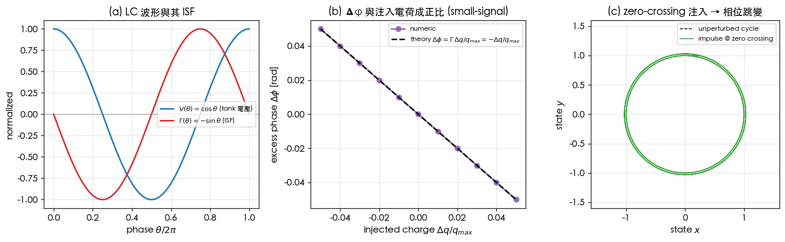
(One three-panel figure: (a) waveform and ISF; (b) $\Delta\phi$ vs $\Delta q$ linearity; (c) state-space zero-crossing injection.)

9. How to read the figures

(a) Waveform and ISF:

• Blue: $V(\theta)=\cos\theta$ (tank voltage); red: $\Gamma(\theta)=-\sin\theta$ (ISF).
• Note the $90^\circ$ phase difference between them: $\Gamma=0$ when $V$ is at its peak, $|\Gamma|=1$ when $V$ crosses zero. Physically this is exactly right — the magnitude of the ISF is set by the waveform slope (large slope = large tangential component = phase-sensitive), and the slope of $\cos$ is $-\sin$. This is precisely the picture "the most phase-sensitive instant is the zero crossing, the least sensitive is the peak".

(b) Linearity:

• The purple dots are the persistent $\Delta\phi$ measured from the numerical simulation; the black dashed line is the theory $\Delta\phi=-\Delta q/q_{max}$ (because the injection is at $\Gamma=-1$). They nearly coincide over the entire $\pm0.05$ range — this is seeing-is-believing for the strict small-signal proportionality of $\Delta\phi$ to $\Delta q$, reproducing [P1] Fig. 6.
• The slope is $-1$ (not $+1$), confirming the minus sign of $\Gamma(\pi/2)=-1$.

(c) State space:

• The black dashed line is the unperturbed unit circle; the green curve is the trajectory after being "kicked tangentially at a zero crossing". Key observation: the trajectory radius is essentially unchanged (amplitude untouched), but the phase of the rotation is permanently shifted — this is the "pure phase jump". By contrast, injecting at the peak makes the radius first grow then get pulled back while the phase barely moves (readers can move t_inj to a peak and try).

10. Corresponding paper equations / figures

• Charge → voltage step: [P1] Eq.(9), p.182: $\Delta V=\Delta q/C_{node}$.
• ISF impulse response and convolution: [P1] Eq.(10),(11), p.182:

$$h_\phi(t,\tau)=\frac{\Gamma(\omega_0\tau)}{q_{max}}\,u(t-\tau),\qquad \phi(t)=\frac{1}{q_{max}}\int_{-\infty}^{t}\Gamma(\omega_0\tau)\,i_n(\tau)\,d\tau.$$

• Concept and linearity figures: [P1] Fig. 4 (state-space limit cycle, peak vs zero-crossing injection), Fig. 6 ($\Delta\phi$ linear in $\Delta q$ at small charge — panel (b) of this lab directly reproduces that conclusion), Fig. 7(a) (the LC ISF shape, corresponding to this lab's $-\sin\theta$). The three panels of this lab are redrawn toy concept figures (not point-by-point copies of the paper figures, and not transistor-level).
• Operational ISF definition: $\Delta\phi=\Gamma(\omega_0\tau)\,\Delta q/q_{max}$; the full step-by-step derivation is in impulse_to_phase_shift (Example A: $q_{max}=1$ pC, $\Delta q=1$ fC, $\Gamma=0.5$, $f_0=5$ GHz → $\Delta\phi=5\times10^{-4}$ rad, $\Delta t=15.9$ fs).

11. Limitations and approximations

• Pedagogical toy model, not transistor-level. $\Gamma=-\sin\theta$ is the result for an ideal lossless LC; a real LC has finite $Q$, a waveform with harmonics, and cyclostationary device noise (gated by the operating point), so the actual $\Gamma$ deviates from the clean $-\sin$ and must be extracted with transient/adjoint/Floquet methods (see effective_isf; the related PPV/adjoint material is not among the five downloaded PDFs and is supplemented from standard literature).
• Small-signal / linearization: projecting onto the tangent assumes $\Delta q\ll q_{max}$. Panel (b) sweeps only up to $\pm0.05\,q_{max}$; larger injections bring in AM–PM conversion, change the ISF itself, or even kick the oscillator off the limit cycle.
• Single node, single injection: real circuits have many nodes, each with its own $\Gamma$ and $q_{max}$; multi-node ISF is discussed in isf_definition.
• Numerical integration error: simulate_lc uses fixed-step RK4; the weak $\mu=0.3$ introduces a tiny bias into the phase measurement. This lab averages over the last period to suppress transient residue. extract_isf_by_injection sweeps the full $\Gamma(\theta)$ with a smaller $\Delta q/q_{max}=10^{-3}$; the maximum error against $-\sin\theta$ is about 0.001 (see lab_04).

Key takeaways

• The ideal-LC ISF is analytically derivable: $\Gamma(\theta)=-\sin\theta$ (from the tangential projection of the voltage step).
• $|\Gamma|$ magnitude = waveform slope: most sensitive at zero crossings ($\Gamma=-1$), insensitive at peaks ($\Gamma=0$).
• In the small-signal regime $\Delta\phi=\Gamma\,\Delta q/q_{max}$; simulation confirms linearity with slope $-1$ ([P1] Fig. 6).
• Zero-crossing injection = pure phase jump (state radius unchanged, phase permanently shifted).
• Sources: [P1] Eq.(9),(10),(11), p.182; Fig. 4, 6, 7(a).