β: This English translation is in beta — the Traditional-Chinese original is the authoritative version.

Lab 03 — Ring-oscillator toy model: accumulated-jitter random walk and ISF comparison

lab_02 looked at the phase jump from a single impulse. In the real world noise kicks continuously, so the phase error accumulates step by step. The ring oscillator ($N$ inverter stages connected in a ring, each with delay $\tau_D$) is the cleanest place to watch this, because it has no absolute time reference: every edge (transition) is timed off the previous edge, so earlier errors propagate forever.

This lab does two things: (1) uses an edge-time model to demonstrate the random walk of accumulated jitter $\sigma_{\Delta t}=\kappa\sqrt{\Delta t}$ ([P2] Eq.(8), p.792; κ from Eq.(12), p.793); (2) contrasts the LC's smooth $-\sin\theta$ with the ring's toy ISF — "concentrated at transitions, shrinking with stage count $N$" — and spells out what this toy model can and cannot show.

Physical intuition (conclusion first): every beat (every edge) is kicked by independent noise into a small timing error, and that error adds onto the accumulated edge time and is never corrected (open loop, no reference). Independent small steps accumulating = a random walk: after $m$ steps the position variance is $\propto m$, so the standard deviation is $\propto\sqrt{m}$, i.e. the timing error $\sigma_{\Delta t}\propto\sqrt{\Delta t}$. This is the same thing as "a drunkard's distance from the origin growing as the square root of the number of steps".

1. Learning objectives

• Understand that the ring oscillator has no absolute time reference → every edge's error keeps propagating → a random walk forms.
• Use simulation to see the $\sqrt{\Delta t}$ scaling (slope $1/2$ on log–log axes) of accumulated (long-term) jitter $\sigma_{\Delta t}=\kappa\sqrt{\Delta t}$ ([P2] Eq.(8)).
• Contrast the LC's smooth ISF $-\sin\theta$ ($\Gamma_{rms}=0.707$) with the ring's toy ISF: energy concentrated at transitions, peak height $\sim1/\sqrt N$, and $\Gamma_{rms}$ decreasing as the stage count $N$ increases.
• Delimit the toy model: it shows the mechanisms (random walk, ISF shape difference) but not the real constants (exact values of $\kappa$ and $\Gamma_{rms}$, or the different scaling of correlated noise).

2. Mathematical model

(A) Edge-time random walk. Abstract the ring's output into a sequence of transition times $\{t_k\}$. Ideally each beat lasts one period $T=1/f_0$; in practice each beat picks up an independent Gaussian timing perturbation with standard deviation $\sigma_{edge}$:

$$t_{k}=t_{k-1}+T+\delta_k,\qquad \delta_k\sim\mathcal{N}(0,\sigma_{edge}^2)\ \text{i.i.d.}$$

The perturbation part of the edge-time difference $t_{k+m}-t_k$ over $m$ beats is then $\sum_{j=1}^{m}\delta_j$. Independent terms add → variances add:

$$\operatorname{Var}\!\Big(\sum_{j=1}^{m}\delta_j\Big)=m\,\sigma_{edge}^2 \;\Longrightarrow\; \sigma_{\Delta t}(m)=\sigma_{edge}\sqrt{m}.$$

Converting the step count $m$ into time $\Delta t=mT$ gives [P2] Eq.(8), p.792:

$$\boxed{\;\sigma_{\Delta t}=\kappa\sqrt{\Delta t}\;},\qquad \kappa=\frac{\sigma_{edge}}{\sqrt{T}}.$$

• dimension check: $[\kappa]=[\text{s}]/[\text{s}]^{1/2}=[\text{s}]^{1/2}=\sqrt{\text{s}}$, consistent with the notation table; $\kappa\sqrt{\Delta t}=\sqrt{\text{s}}\cdot\sqrt{\text{s}}=\text{s}$ ✓.
• Key assumption: the per-beat perturbations are mutually independent (uncorrelated). The paper ([P2] Sec. III, p.793) explicitly distinguishes: uncorrelated sources such as thermal noise → variances add → $\sigma\propto\sqrt{\Delta t}$ (this lab); versus fully correlated sources such as substrate/supply/$1/f$ → standard deviations add → $\sigma\propto\Delta t$ (this toy model does not simulate that branch; see Section 11).

(B) Ring vs LC ISF shape. The ring's energy is concentrated at the transitions (the switching instant has the largest slope and is the most sensitive); its ISF is not the LC's smooth $-\sin$ but has a spike near every transition. This lab uses a triangular toy ISF to "sketch" this, with peak height shrinking with stage count $N$:

$$\Gamma_{ring}^{toy}(\theta)\propto\frac{1}{\sqrt N}\times(\text{每半週期一個三角脈衝}).$$

This echoes the $\Gamma_{rms}\propto N^{-3/2}$ scaling trend claimed by [P2] (more stages → each stage contributes less to the total phase).

Toy-model note: both parts are pedagogical toy models, not transistor-level. The random walk uses abstract per-edge Gaussian perturbations (not computed from device thermal noise); the triangular ISF is only an illustration of "energy concentrated at transitions", not an extracted ring ISF — the constants await verification against a real extraction.

3. Block diagram

4. Core Python code

Excerpted from simulations/lab_03_ring_toy_model.py (checked against the source). Accumulated jitter uses accumulated_jitter_curve (internally a cumsum of per-period Gaussian increments over n_trials trials, i.e. a random walk); the ISF comparison uses gamma_lc_ideal, gamma_triangular, and gamma_rms:

from oscillator_models import accumulated_jitter_curve
from simulations.common.isf_utils import gamma_lc_ideal, gamma_triangular, gamma_rms

RNG = np.random.default_rng(12345)

def fig_accumulation():
    f0 = 5e9              # 5 GHz
    sigma_edge = 50e-15   # independent timing perturbation, 50 fs rms per beat
    # cumsum of per-period Gaussian increments over 2000 trials -> random walk
    lags, sigma_dt = accumulated_jitter_curve(
        f0, sigma_edge, max_lag_periods=500, n_trials=2000, rng=RNG)
    # simulated points vs theory sigma_edge*sqrt(lags): a slope-1/2 line on log-log axes

def fig_lc_vs_ring_isf():
    theta = np.linspace(0, 2 * np.pi, 1000, endpoint=True)
    g_lc  = gamma_lc_ideal(theta)               # -sin(theta), smooth
    g_r5  = gamma_triangular(theta, n_stages=5)  # toy triangle, peak height ~ 1/sqrt(5)
    g_r15 = gamma_triangular(theta, n_stages=15) # toy triangle, peak height ~ 1/sqrt(15)
    # gamma_rms(theta, g_lc)=0.707, g_r5=0.258, g_r15=0.149 -> rms drops as N rises

The core of accumulated_jitter_curve is just walk = np.cumsum(incr, axis=1) followed by np.std across trials — it directly measures "the variance of a random walk grows linearly with the step count".

5. Full script path

simulations/lab_03_ring_toy_model.py (depends on accumulated_jitter_curve (and ring_edge_times) from simulations/common/oscillator_models.py; gamma_lc_ideal, gamma_triangular, gamma_rms from simulations/common/isf_utils.py; savefig from simulations/common/plot_utils.py.)

To run: python scripts/run_all_sims.py or python simulations/lab_03_ring_toy_model.py.

6. Parameter table

Parameter	Code variable	Value	Meaning
Oscillation frequency	f0	$5\times10^{9}$ Hz (5 GHz)	matches the site-wide canonical $f_0$
Per-beat timing perturbation	sigma_edge	$50\times10^{-15}$ s (50 fs)	rms of the independent per-beat Gaussian perturbation
Maximum measurement interval	max_lag_periods	500 periods ($=100$ ns @ 5 GHz)	longest accumulated lag
Trial count	n_trials	2000	Monte-Carlo statistical samples
Random seed	RNG	12345	reproducible results
LC ISF	gamma_lc_ideal	$-\sin\theta$	$\Gamma_{rms}=0.707$
ring toy ISF (N=5)	gamma_triangular(.,5)	peak height $1/\sqrt5$	$\Gamma_{rms}=0.258$
ring toy ISF (N=15)	gamma_triangular(.,15)	peak height $1/\sqrt{15}$	$\Gamma_{rms}=0.149$

7. Units table

Quantity	Symbol	Unit	Note
Measurement interval	$\Delta N$ (periods) / $\Delta t$ (seconds)	periods / s	$\Delta t=\Delta N\cdot T$
Accumulated jitter	$\sigma_{\Delta t}$	s (fs in the plot)	rms
Per-beat perturbation	$\sigma_{edge}$	s	50 fs
Proportionality constant	$\kappa$	$\sqrt{\text{s}}$	$\kappa=\sigma_{edge}/\sqrt T$
Phase	$\theta$	rad	ISF argument
ISF	$\Gamma(\theta)$	dimensionless	LC vs ring comparison
rms ISF	$\Gamma_{rms}$	dimensionless	$\sqrt{\frac{1}{2\pi}\int_0^{2\pi}\Gamma^2\,d\theta}$
Stage count	$N$	dimensionless	number of ring inverter stages

8. Simulation figures

(Figure 1) The √Δt random walk of accumulated jitter

(Figure 2) LC vs ring ISF comparison

9. How to read the figures

Figure 1 (accumulated jitter, log–log):

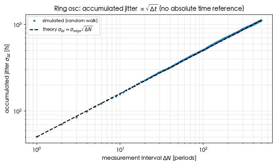
• Blue dots: $\sigma_{\Delta t}$ simulated over 2000 trials; black dashed line: the theory $\sigma_{\Delta t}=\sigma_{edge}\sqrt{\Delta N}$. They collapse onto a single line of slope $1/2$ (on log–log axes, $\sqrt{}$ is slope $1/2$) — the fingerprint of a random walk.
• Numerical feel: $\sigma_{edge}=50$ fs; after 1 beat $\sigma=50$ fs; after 500 beats $\sigma=50\times\sqrt{500}\approx1118$ fs $\approx1.12$ ps (@ 5 GHz, 500 beats $=100$ ns). Stretching the measurement time by 100× (1→100 beats) grows the jitter only $\sqrt{100}=10$× — this is "why an open-loop oscillator drifts further the longer it runs, but drifts ever more slowly".
• Contrast: with a locked PLL there is an absolute reference and the accumulation is truncated (outside the scope of this toy).

Figure 2 (ISF comparison):

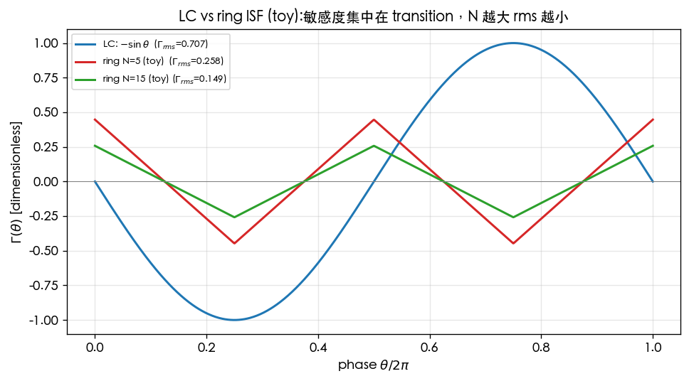
• Blue: the LC's $-\sin\theta$ — smooth, $\Gamma_{rms}=0.707$. Red (N=5) and green (N=15): the ring's toy triangular ISFs: energy concentrated at transitions (one spike per half period), with peaks getting shorter and shorter.
• Read-off $\Gamma_{rms}$: LC $=0.707$, ring N=5 $=0.258$, ring N=15 $=0.149$. Larger stage count $N$ → smaller $\Gamma_{rms}$ — qualitatively echoing [P2]'s $\Gamma_{rms}\propto N^{-3/2}$ trend (more stages, each stage's weight in the total phase gets diluted). Since $1/f^2$ phase noise $\propto\Gamma_{rms}^2/q_{max}^2$ ([P1] Eq.(21)), this explains "how the ring's stage count / power budget affects phase noise at design time" (see lc_vs_ring).
• Note: the toy triangle's absolute peak height and the precise $N^{-3/2}$ coefficient are not verified by real extraction — the trend is illustrative only.

10. Corresponding paper equations / figures

• Accumulated jitter (core): [P2] Eq.(8), p.792:

$$\sigma_{\Delta t}=\kappa\sqrt{\Delta t}.$$

The narrative in [P2] Sec. III (p.793) states explicitly that because "uncertainty in any earlier transition affects all following transitions, and its effect persists indefinitely", variances add for uncorrelated sources and $\sigma\propto\sqrt{\Delta t}$; Figure 1 of this lab directly reproduces this equation (compare the "rms jitter vs measurement time, log–log" concept of [P2] Fig. 3 and Fig. 4).

• The other branch — correlated sources: the same section of [P2] notes that for correlated sources (substrate/supply/$1/f$) standard deviations add, $\sigma\propto\Delta t$ (slope 1, not 1/2). This toy simulates uncorrelated only.
• Ring frequency (background): [P2] Eq.(15), p.794: $f_0=\dfrac{1}{2N\tau_D}$.
• $\Gamma_{rms}$ scaling: [P2] Eq.(16), p.794: $\Gamma_{rms}\propto N^{-3/2}$ ([P2] Eq.(16), p.794 — v7 re-verified: the square root covers only the constant, so $\Gamma_{rms}\propto N^{-3/2}$; the body text's $4/N^{1.5}$ at η=0.75 and App. B Eq.(55) triple-confirm this. v3 had misread it as $N^{-3/4}$; this lab echoes it only qualitatively; compare $\Gamma_{rms}$ vs $N$ in [P2] Fig. 8). Both figures of this lab are redrawn toy concept figures (not point-by-point copies of the paper figures, not transistor-level).
• Link to phase noise: $\Gamma_{rms}$ enters $1/f^2$ phase noise through [P1] Eq.(21), p.185.

11. Limitations and approximations — what the toy model can and cannot show

Can show (mechanisms this toy model teaches correctly):

• An open-loop oscillator has no absolute time reference → errors propagate forever → the random-walk nature of accumulated jitter.
• Under uncorrelated noise, $\sigma_{\Delta t}\propto\sqrt{\Delta t}$ (log–log slope $1/2$).
• The qualitative shape of the ring ISF — energy concentrated at transitions — contrasted with the LC's smooth $-\sin$.
• The direction of the trend that $\Gamma_{rms}$ shrinks as $N$ grows.

Cannot show (things the toy model misses; need transistor-level / real extraction):

• The real $\kappa$ and $\sigma_{edge}$: the 50 fs in this lab is a hand-placed number, not computed from device thermal noise + $\Gamma$ + $q_{max}$ (that requires [P1] Eq.(21) and the real ISF).
• The different scaling of correlated noise: substrate/supply/$1/f$ give $\sigma\propto\Delta t$ (slope 1); this model contains none of that branch — a real ring shows both trends ([P2] Sec. III).
• The precise $\Gamma_{rms}\propto N^{-3/2}$ constant and the real ring ISF shape: the triangle is only illustrative; the real ISF must be extracted via transient/adjoint methods (the related PPV/adjoint/Floquet material is not among the five downloaded PDFs and is supplemented from standard literature; see effective_isf).
• Flicker ($1/f$) upconversion and cyclostationarity: the per-edge perturbations in this lab are pure white and symmetric, with no $1/f^3$ close-in behavior (see lab_07).
• Small-lag saturation: a footnote in [P2] notes that under a more accurate treatment the phase noise does not grow without bound as $f_0\to0$ (it flattens); this random walk contains no such correction at large lag — but, as the paper says, it makes "no practical difference" for this discussion.

Key takeaways

• The ring has no absolute time reference → errors propagate forever → accumulated jitter is a random walk.
• Uncorrelated noise: $\sigma_{\Delta t}=\kappa\sqrt{\Delta t}$ ([P2] Eq.(8)); simulated log–log slope $1/2$; 50 fs/beat → 500 beats ≈ 1.12 ps.
• Correlated noise instead gives $\sigma\propto\Delta t$ (not included in this toy).
• The ring ISF is concentrated at transitions with peak height $\sim1/\sqrt N$; $\Gamma_{rms}$ (LC 0.707 → ring N=5 0.258 → N=15 0.149) drops with $N$, echoing $\Gamma_{rms}\propto N^{-3/2}$.
• Sources: [P2] Eq.(8),(14),(16), Sec. III, Fig. 3,4,8; linked to [P1] Eq.(21).