β: This English translation is in beta — the Traditional-Chinese original is the authoritative version.

Lab 06 — White Noise → 1/f² Phase Noise

This lab runs the entire causal chain — white noise → ISF weighting → integration → phase — in the cleanest possible numerical form, so you can see with your own eyes how a flat (white, frequency-independent) current-noise power spectrum gets colored by the oscillator — a "phase integrator" — into $1/f^2$ ($-20$ dB per decade) phase noise.

Physical intuition (conclusion first): the oscillator's phase has no restoring force (a force that pulls a perturbation back), so every phase step kicked in by noise accumulates permanently — this is an integrator (a system that time-integrates its input; infinite memory). The integrator's transfer-function magnitude is $1/(2\pi f)$, which is $1/(2\pi f)^2$ for a PSD. The input is flat (white noise), so the output is multiplied by $1/f^2$. White in, $1/f^2$ out — not because the noise source is $1/f^2$, but because phase is obtained by integration.

1. Learning objectives

• Verify by simulation the signature result of [P1]: white current noise becomes $1/f^2$ phase noise in an oscillator.
• Understand where the $-20$ dB/decade slope comes from (the integrator, not the noise source).
• Quantitatively verify the theoretical prediction $S_\phi(f)=\Gamma_{rms}^2 S_i/(q_{max}^2(2\pi f)^2)$.
• Understand the famous factor-of-2 controversy: the clean time-domain derivation differs from [P1] Eq.(21) by a factor of 2, but the scaling and slope are entirely unaffected.

2. Mathematical model

The phase response is the LTV (linear time-variant) convolution expression [P1] Eq.(11), p.182:

$$\phi(t)=\frac{1}{q_{max}}\int_{-\infty}^{t}\Gamma(\omega_0\tau)\,i_n(\tau)\,d\tau$$

Split it into three blocks: first phase-weight the noise with the ISF, then integrate. The input is white current noise with constant one-sided PSD (power spectral density) $S_i$ ($A^2/$Hz).

Integrating the white input, the clean time-domain result for the output phase PSD is

$$S_\phi(f)=\frac{\Gamma_{rms}^2\,S_i}{q_{max}^2\,(2\pi f)^2}.$$

• Where it comes from: after the ISF weights the white noise, the average power is scaled by $\Gamma_{rms}^2$ (the ISF's rms squared, see [P1] Eq.(20)), with $q_{max}^2$ in the denominator (normalization); the integrator is then $1/(j2\pi f)$ in the frequency domain, i.e. $1/(2\pi f)^2$ for the PSD.
• Dimension check: $\Gamma_{rms}^2$ is dimensionless, $S_i$ is $A^2/$Hz, $q_{max}^2$ is $C^2$, $(2\pi f)^2$ is $(\text{rad/s})^2=\text{s}^{-2}$. Overall $=\dfrac{A^2/\text{Hz}}{C^2\cdot\text{s}^{-2}}=\dfrac{A^2\,\text{s}^2}{C^2}\cdot\dfrac{1}{\text{Hz}}$. Since $C=A\cdot s$, $A^2 s^2/C^2=1$ (dimensionless = rad²), so $[S_\phi]=\text{rad}^2/\text{Hz}$ ✓.

This has the same scaling as the signature expression [P1] Eq.(21), p.185:

$$\mathcal{L}\{\Delta\omega\}=10\log_{10}\!\left(\frac{\Gamma_{rms}^2}{q_{max}^2}\cdot\frac{\overline{i_n^2}/\Delta f}{4\,\Delta\omega^2}\right)$$

factor-of-2 teaching note (must read): the clean time-domain derivation "white noise × ISF → integrate" gives $S_\phi=\Gamma_{rms}^2 S_i/(q_{max}^2(2\pi f)^2)$, corresponding to SSB $\mathcal{L}=\Gamma_{rms}^2 S_i/(2q_{max}^2\Delta\omega^2)$ (denominator $2$); whereas [P1] Eq.(21) is written with denominator $4\Delta\omega^2$. This factor of 2 comes from the SSB (single-sideband) bookkeeping convention — a famous minor controversy in the literature. It does not affect the $\Gamma_{rms}^2/q_{max}^2$ scaling, nor the $-20$ dB/decade slope — those are the physics. The simulation in this lab uses the clean time-domain version (denominator $(2\pi f)^2$), so the simulated curve sits on the time-domain theory line. See white_noise_to_phase_noise.

3. Block diagram

4. Core Python code

Verbatim from main() in simulations/lab_06_white_noise_phase_noise.py: three steps (generate white noise → ISF weighting → cumsum integration), then Welch-estimate the phase PSD and overlay the theory line.

f0 = 1.0
fs = 256.0                 # 256 samples per period
n = 2 ** 20                # ~4096 periods -> good low-freq resolution
t = np.arange(n) / fs

q_max = 1.0
S_i = 1.0e-4               # one-sided white current PSD [A^2/Hz] (normalized)

# ISF and its rms
theta_grid = np.linspace(0, 2 * np.pi, 4000, endpoint=True)
Grms = gamma_rms(theta_grid, gamma_lc_ideal(theta_grid))  # = 1/sqrt(2)

# 1) white current noise
i_n = white_noise(n, psd=S_i, fs=fs, rng=RNG)
# 2) ISF weighting
g = gamma_lc_ideal(2 * np.pi * f0 * t) * i_n / q_max
# 3) integrate (cumulative) -> excess phase
dt = 1.0 / fs
phi = np.cumsum(g) * dt
phi = phi - np.mean(phi)   # remove the random-walk DC offset for PSD est.

# 4) estimate phase PSD
f, Sphi = estimate_psd(phi, fs, nperseg=2 ** 16)

# theory line
Sphi_theory = Grms ** 2 * S_i / (q_max ** 2 * (2 * np.pi * f) ** 2)

• Step 3, np.cumsum(g) * dt, discretizes the $\int d\tau$ in the convolution expression — the cumulative sum is the integrator, i.e. the source of the phase's "infinite memory".
• The ISF is the ideal-LC gamma_lc_ideal ($\Gamma(\theta)=-\sin\theta$), whose $\Gamma_{rms}=1/\sqrt2\approx0.707$ (because $\langle\sin^2\rangle=1/2$).

5. Full script path

simulations/lab_06_white_noise_phase_noise.py (Dependencies: white_noise and estimate_psd from simulations/common/noise_utils.py; gamma_lc_ideal and gamma_rms from simulations/common/isf_utils.py.)

How to run: python scripts/run_all_sims.py (generates all figures into static/figures/).

6. Parameter table

Parameter	Variable	Value	Notes
Oscillation frequency	f0	$1.0$ (normalized)	the whole lab uses $f_0=1$ normalization; absolute dBc/Hz is computed in lab_08
Sampling rate	fs	$256$	256 samples per period
Number of samples	n	$2^{20}=1{,}048{,}576$	about 4096 periods, sufficient low-frequency resolution
Maximum charge swing	q_max	$1.0$	for normalization
White current-noise PSD	S_i	$1\times10^{-4}$	one-sided, frequency-independent
ISF	gamma_lc_ideal	$-\sin\theta$	ideal LC, $\Gamma_{rms}=1/\sqrt2$
PSD segment length	nperseg	$2^{16}=65{,}536$	Welch segmentation, traded for low-frequency resolution
Random seed	RNG	default_rng(2024)	reproducible results

7. Units table

Quantity	Symbol	Unit (normalized lab)
Time	$t$	s (in units of the "period" when $f_0=1$)
Current-noise PSD	$S_i$	A²/Hz
Maximum charge swing	$q_{max}$	C
ISF	$\Gamma(\omega_0\tau)$	dimensionless
ISF rms	$\Gamma_{rms}$	dimensionless
Excess phase	$\phi(t)$	rad
Phase PSD	$S_\phi(f)$	rad²/Hz
Offset frequency	$f$	Hz (normalized, $f_0=1$)

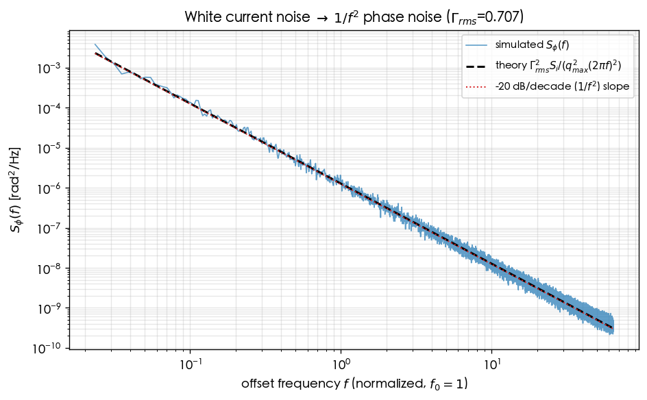
8. Simulation figure

9. How to read the figure

• Blue line (simulated $S_\phi$): the PSD actually estimated from the simulated phase sequence. On log–log it is a straight line of slope $-2$ (dropping $20$ dB per decade), with the random fluctuations of a Welch estimate.
• Black dashed line (theory): the analytic line $\Gamma_{rms}^2 S_i/(q_{max}^2(2\pi f)^2)$. The blue line hugs the black one — this is "white noise → $1/f^2$" confirmed numerically.
• Red dotted line ($-20$ dB/dec guide): a pure slope reference confirming the slope is exactly $-2$.
• Key point: the input is flat ($S_i$ independent of $f$), yet the output is $1/f^2$. The extra $1/f^2$ comes entirely from the integrator in step 3. Swapping in a different ISF shape only changes $\Gamma_{rms}$ (shifting the whole line up or down); the slope is always $-2$. The height of the whole line is set by $\Gamma_{rms}^2/q_{max}^2$, so enlarging $q_{max}$ (tank swing) is the main knob for lowering $1/f^2$ phase noise (design usage in tank_swing).

Plugging in this lab's numbers as a sanity check: $\Gamma_{rms}^2=0.5$, $S_i=10^{-4}$, $q_{max}=1$; at $f=0.1$ (normalized), $2\pi f=0.6283$, $(2\pi f)^2=0.3948$, $S_\phi=0.5\times10^{-4}/0.3948=1.27\times10^{-4}$ rad²/Hz. The height of the plot at $f=0.1$ should be of this order.

10. Corresponding paper equations/figures

• Theory-line source: the clean time-domain version $S_\phi=\Gamma_{rms}^2 S_i/(q_{max}^2(2\pi f)^2)$, matching the scaling of [P1] Eq.(21), p.185 (differs by the factor-of-2, see the note above).
• $\Gamma_{rms}$ definition: [P1] Eq.(20), p.185, $\sum_{n=0}^{\infty}c_n^2=\frac{1}{\pi}\int_0^{2\pi}|\Gamma(x)|^2dx=2\Gamma_{rms}^2$.
• White-noise sum expression: [P1] Eq.(19), p.185, $\mathcal{L}=10\log_{10}\big(\frac{\overline{i_n^2}/\Delta f\sum_n c_n^2}{8q_{max}^2\Delta\omega^2}\big)$; substituting Eq.(20) to replace $\sum c_n^2$ with $2\Gamma_{rms}^2$ yields Eq.(21).
• Concept-figure source: paper_001 Eq.(21) (the factor-of-2 SSB note lives in this lab). Corresponding site figure white_noise_phase_noise_psd.png.

11. Limitations and approximations

• This is a pedagogical toy model, not transistor-level: the ISF is the analytic $-\sin\theta$ (ideal LC), not extracted from a real circuit. $q_{max}=1$, $f_0=1$ are normalized units, so there is no absolute dBc/Hz (for absolute values see lab_08 and numerical_feeling example B).
• Single white-noise source, stationary assumption: real circuits have multiple sources and are cyclostationary (noise intensity varies periodically with the operating point); the correction is $\Gamma_{eff}=\Gamma\cdot\alpha$ (see effective_isf).
• Small-angle approximation: phase is treated as linearly superposable and small; for large phase excursions $\mathcal{L}\approx\frac12 S_\phi$ breaks down.
• factor-of-2: the simulation agrees with the time-domain theory line (denominator $(2\pi f)^2$) and differs from the $4\Delta\omega^2$ of [P1] Eq.(21) by the SSB-bookkeeping factor of 2 — slope and scaling unaffected.
• Numerical limits: the low-frequency end is limited by the total simulated time ($\approx4096$ periods) and nperseg; the leftmost few points have larger statistical scatter, and the plot shows only the trustworthy region $f>0.02$.

Key takeaways

• White noise (flat) → ISF weighting (scale by $\Gamma_{rms}^2/q_{max}^2$) → integrator (multiply by $1/(2\pi f)^2$) → $1/f^2$ phase noise.
• The $-20$ dB/decade slope comes from the integrator, independent of the noise source's spectral shape.
• The simulated PSD hugs the theory line $\Gamma_{rms}^2 S_i/(q_{max}^2(2\pi f)^2)$.
• The factor-of-2 is an SSB bookkeeping-convention difference; it changes neither the scaling nor the slope.

Further reading

• Full theory derivation: white_noise_to_phase_noise
• Origin of the convolution/integrator: convolution_derivation
• Next lab (1/f upconversion): lab_07_flicker_noise_upconversion
• Converting to absolute jitter: lab_08_jitter_integration
• Use in design/theory: suppress $1/f^2$ with $q_{max}$ (tank swing) → tank_swing