β: This English translation is in beta — the Traditional-Chinese original is the authoritative version.

Lab 08 — rms Jitter by Integrating L(f)

This lab turns something you see on every datasheet — the single-sideband phase-noise curve $\mathcal{L}(f)$ (dBc/Hz) — into the number designers actually care about: rms timing jitter $\sigma_t$. We use a canonical scenario ($f_0=5$ GHz, $\mathcal{L}(1\text{MHz})=-100$ dBc/Hz, $1/f^2$ slope, integrated 1→100 MHz) and make the numerical integration and the analytic closed form agree digit by digit: $\sigma_t=447.9$ fs.

Physical intuition (conclusion first): phase noise is "how much phase power density sits at each offset frequency"; jitter is "add it all up, take the square root, convert to time". So going from $\mathcal{L}(f)$ to $\sigma_t$ is three things: (1) convert dBc/Hz back to linear and multiply by 2 to recover $S_\phi$; (2) integrate over offset frequency to get the phase variance; (3) take the square root and divide by $2\pi f_0$ to convert to time. For a $1/f^2$ shape, the integral is dominated by the lower limit $f_1$ — "where you start integrating" matters far more than "how high you go".

1. Learning objectives

• Convert $\mathcal{L}(f)$ (dBc/Hz) step by step into rms phase $\sigma_\phi$ and rms jitter $\sigma_t$.
• Build a feel for the 5 GHz conversion: $-100$ dBc/Hz @ 1 MHz, $1/f^2$, integrated 1→100 MHz → about 448 fs.
• Verify numerical integration = analytic closed form ($1/f^2$ has a closed form).
• Understand why $1/f^2$ jitter is dominated by the lower integration limit.

2. Mathematical model

Step 1: $\mathcal{L}$ → $S_\phi$. Under the small-angle / single-sideband approximation (canonical formula 16):

$$\mathcal{L}(\Delta f)\approx\tfrac12 S_\phi(\Delta f)\;\Rightarrow\;S_\phi(f)=2\cdot10^{\mathcal{L}(f)/10}.$$

Step 2: write the $1/f^2$ shape (anchored at $f_{ref}=1$ MHz, canonical example C):

$$S_\phi(f)=S_\phi(f_{ref})\left(\frac{f_{ref}}{f}\right)^2.$$

Step 3: integrate to get the phase variance (canonical formula 18):

$$\sigma_\phi^2=\int_{f_1}^{f_2}S_\phi(f)\,df.$$

For the $1/f^2$ shape this integral has a closed form ($\int f^{-2}df=-1/f$):

$$\sigma_\phi^2=S_\phi(f_{ref})\,f_{ref}^2\!\int_{f_1}^{f_2}\frac{df}{f^2}=S_\phi(f_{ref})\,f_{ref}^2\left(\frac{1}{f_1}-\frac{1}{f_2}\right).$$

Step 4: convert to rms jitter (canonical formula 19):

$$\sigma_t=\frac{\sigma_\phi}{2\pi f_0}=\frac{1}{2\pi f_0}\sqrt{\int_{f_1}^{f_2}S_\phi(f)\,df}.$$

• Dimension check (step 4): $\sigma_\phi$ is rad, $2\pi f_0$ is rad/s, $[\text{rad}]/[\text{rad/s}]=[\text{s}]$ ✓.
• Lower-limit dominance: $\big(\tfrac1{f_1}-\tfrac1{f_2}\big)=10^{-6}-10^{-8}=9.9\times10^{-7}$, of which $1/f_1=10^{-6}$ contributes 99%. So the integral depends almost entirely on $f_1$.

Substituting the canonical numbers digit by digit (identical to numerical_feeling example C):

$$\begin{aligned} S_\phi(1\text{MHz})&=2\times10^{-100/10}=2\times10^{-10}\ \text{rad}^2/\text{Hz},\\ \sigma_\phi^2&=2\times10^{-10}\,(10^6)^2\,(10^{-6}-10^{-8})=200\times9.9\times10^{-7}=1.98\times10^{-4}\ \text{rad}^2,\\ \sigma_\phi&=1.407\times10^{-2}\ \text{rad}=14.07\ \text{mrad},\\ \sigma_t&=\frac{1.407\times10^{-2}}{2\pi\times5\times10^{9}}=4.479\times10^{-13}\ \text{s}=447.9\ \text{fs}. \end{aligned}$$

3. Block diagram

4. Core Python code

Verbatim from main() in simulations/lab_08_jitter_integration.py: first build the $1/f^2$ curve with leeson_one_over_f2, then integrate numerically with integrate_rms_jitter, and finally check against the hand-computed $1/f^2$ closed form.

import numpy as np
from simulations.common.noise_utils import leeson_one_over_f2, integrate_rms_jitter

f0 = 5e9
f_ref = 1e6
L_ref = -100.0  # dBc/Hz
f1, f2 = 1e6, 100e6

f = np.logspace(np.log10(f1), np.log10(f2), 4000)
L = leeson_one_over_f2(f, L_ref, f_ref)

# numerical integration
sigma_t, sigma_phi = integrate_rms_jitter(f, L, f0, f1, f2)

# analytic closed form (1/f^2)
L_ref_lin = 10 ** (L_ref / 10)
sigma_phi2_analytic = 2 * L_ref_lin * f_ref ** 2 * (1 / f1 - 1 / f2)
sigma_phi_analytic = np.sqrt(sigma_phi2_analytic)
sigma_t_analytic = sigma_phi_analytic / (2 * np.pi * f0)

print(round(sigma_t * 1e15, 1))    # -> 447.9   (sigma_t in fs)
print(round(sigma_phi * 1e3, 2))   # -> 14.07   (sigma_phi in mrad)

The underlying function integrate_rms_jitter (noise_utils.py) implements exactly steps 1, 3, and 4:

l_linear   = 10 ** (l_dbc_per_hz[mask] / 10)   # dBc/Hz -> linear
s_phi      = 2 * l_linear                       # L ~= 0.5 * S_phi
sigma_phi  = np.sqrt(_trapz(s_phi, f[mask]))    # integrate + square root
sigma_t    = sigma_phi / (2 * np.pi * f0)        # convert to time

• The script prints sigma_phi (numeric) ≈ sigma_phi (analytic) and sigma_t ≈ 447.9 fs; the numerical and analytic values agree digit by digit (the only difference is the negligible discretization error of logspace sampling and trapezoidal integration).

5. Full script path

simulations/lab_08_jitter_integration.py (Dependencies: leeson_one_over_f2 and integrate_rms_jitter from simulations/common/noise_utils.py.)

How to run: python scripts/run_all_sims.py.

6. Parameter table

Parameter	Variable	Value	Notes
Oscillation frequency	f0	$5\times10^{9}$ Hz	5 GHz carrier
Reference offset	f_ref	$1\times10^{6}$ Hz	1 MHz, anchor point
Reference phase noise	L_ref	$-100$ dBc/Hz	single datasheet-style number
Lower integration limit	f1	$1\times10^{6}$ Hz	1 MHz (dominates the integral)
Upper integration limit	f2	$100\times10^{6}$ Hz	100 MHz
Number of sample points	—	$4000$ (logspace)	log-uniform sampling
Slope	—	$1/f^2$ ($-20$ dB/dec)	pure skirt

7. Units table

Quantity	Symbol	Unit	Result in this lab
Phase noise	$\mathcal{L}(f)$	dBc/Hz	$-100$ @ 1 MHz
Phase PSD	$S_\phi(f)$	rad²/Hz	$2\times10^{-10}$ @ 1 MHz
Phase variance	$\sigma_\phi^2$	rad²	$1.98\times10^{-4}$
rms phase	$\sigma_\phi$	rad	$14.07$ mrad
rms jitter	$\sigma_t$	s	$447.9$ fs
Offset frequency	$f$	Hz	1–100 MHz
Carrier frequency	$f_0$	Hz	5 GHz

8. Simulation figure

9. How to read the figure

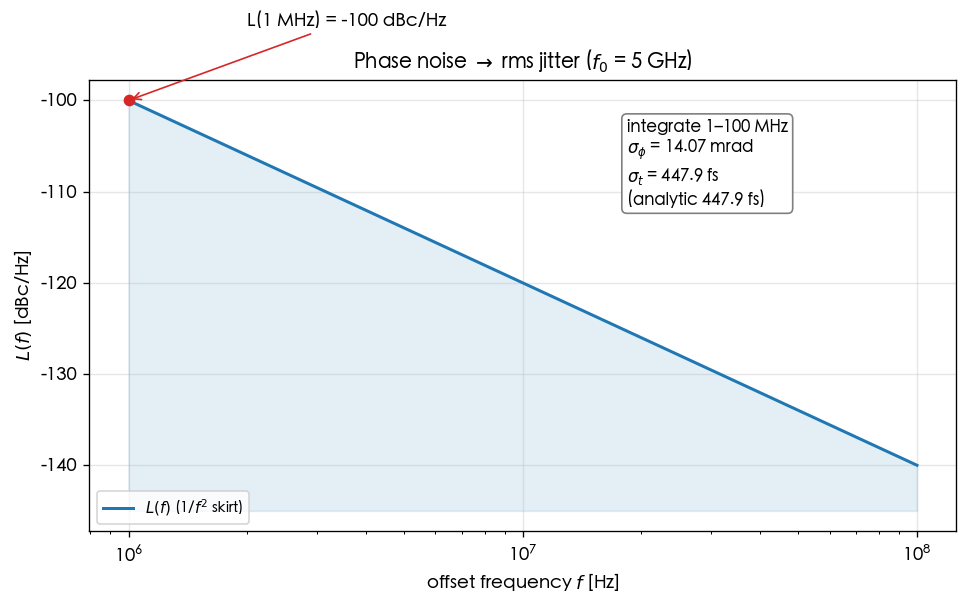
• Blue line ($L(f)$): a straight line on semilog (logarithmic x-axis), because $1/f^2$ has a constant slope in dBc/Hz vs log-f ($-20$ dB/dec). The red dot marks the anchor point $\mathcal{L}(1\text{MHz})=-100$ dBc/Hz.
• Blue shading: illustrates "where the phase power sits over offset frequency". Under $1/f^2$, the part closest to $f_1$ contributes the most — the visual rendering of "lower-limit dominance".
• Text box: lists the integration results $\sigma_\phi=14.07$ mrad, $\sigma_t=447.9$ fs, and notes that the analytic value equals the numerical one, proving the closed form matches the trapezoidal integration.
• How to use it: take any datasheet $\mathcal{L}(f)$ curve, integrate the area under the blue line, take the square root, divide by $2\pi f_0$, and you have the jitter. Remember the 5 GHz conversion point: $\approx448$ fs in this example. With phase noise 20 dB better ($-120$ dBc/Hz @ 1 MHz), the power is 100× smaller and $\sigma$ 10× smaller → $\approx45$ fs.

10. Corresponding paper equations/figures

• This lab uses the standard jitter integration (canonical formulas 16–19), general DSP/communications practice — not among the five source PDFs, supplemented from standard references; consistent in spirit with the jitter discussion in [P2] (period/accumulated jitter).
• $\mathcal{L}\approx\frac12 S_\phi$: canonical formula 16 (small-angle approximation).
• Phase variance: canonical formula 18, $\sigma_\phi^2=\int_{f_1}^{f_2}S_\phi df$.
• rms jitter: canonical formula 19, $\sigma_t=\frac{1}{2\pi f_0}\sqrt{\int S_\phi df}$.
• Concept-figure source: standard jitter integration / SerDes practice. Corresponding site figure phase_noise_to_jitter_integration.png, also cited in numerical_feeling example C, psd_phase_noise_jitter, and serdes_clocking_connection.

11. Limitations and approximations

• Small-angle approximation $\mathcal{L}\approx\frac12 S_\phi$: breaks down at large phase excursions; here $\sigma_\phi=14$ mrad $\ll1$ rad, so the approximation is excellent.
• Pure $1/f^2$ skirt assumption: real curves also have $1/f^3$ (close-in, see lab_07) and a far-out white floor (noise floor). This lab takes only a single $1/f^2$ segment — a teaching simplification. This part is not a toy (the integration flow itself is real engineering practice), but the $L(f)$ shape is idealized.
• Sensitivity to the integration range: with $1/f^2$, the lower limit $f_1$ dominates; changing $f_1$ visibly changes $\sigma_t$, while the upper limit matters little. In practice $f_1$, $f_2$ must be chosen per application (PLL loop bandwidth, data rate).
• Numerical = analytic: the two differ only by the discretization error (logspace + trapezoidal rule), negligible in this setup.

Key takeaways

• $\mathcal{L}$ (dBc/Hz) → linear → $\times2$ gives $S_\phi$ → integrate → square root → $\div(2\pi f_0)$ = rms jitter.
• Canonical: 5 GHz, $-100$ dBc/Hz @ 1 MHz, $1/f^2$, integrated 1→100 MHz → $\sigma_\phi=14.07$ mrad, $\sigma_t=447.9$ fs.
• $1/f^2$ jitter is dominated by the lower integration limit (the $1/f_1$ term).
• The numerical integration agrees digit by digit with the $1/f^2$ analytic closed form.

Further reading

• Same problem, mental-math version: numerical_feeling (example C)
• PSD and jitter types: psd_phase_noise_jitter
• Origin of close-in $1/f^3$: lab_07_flicker_noise_upconversion
• Use in design/theory: how rms jitter sets the eye and BER → serdes_clocking_connection