β: This English translation is in beta — the Traditional-Chinese original is the authoritative version.

Lab 10 — how phase noise smears the carrier into an RF skirt

Breadcrumb: Simulation labs › Noise & jitter › This page (RF spectrum skirt). Upstream: white_noise_to_phase_noise; downstream: lab_08.

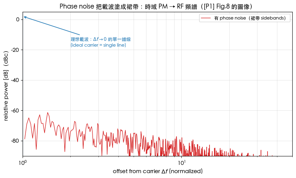
This lab connects the abstract phase-noise PSD $S_\phi(f)$ to what you actually see on a spectrum analyzer: an ideal carrier is a single line in the spectrum; with phase noise, that line gets "smeared" into a continuous skirt (sidebands sloping down on both sides of the carrier). We synthesize $v(t)=\cos(\omega_0 t+\phi(t))$ directly in the time domain, take an FFT, and see it with our own eyes — this is exactly the picture in [P1] Fig. 8, and it's where the unit dBc/Hz (decibels relative to carrier per Hz) comes from.

Physical intuition (conclusion first): phase noise is not "an extra noise source sitting next to the carrier" — it is the carrier's own phase jittering. Stuff the jittering phase $\phi(t)$ into the cosine's phase argument (phase modulation, PM), and the carrier's energy "leaks" from that one clean spectral line into nearby offset frequencies. How far it leaks and how much depends on the spectral shape of $\phi(t)$: $1/f^2$ phase noise → a skirt that falls off at $-20$ dB/dec on either side of the carrier. Seeing the skirt means seeing $S_\phi(f)$ "moved" next to the carrier.

1. Learning objectives

• Start from the time-domain PM signal $v(t)=\cos(\omega_0 t+\phi(t))$ and use an FFT to see the sideband skirt caused by phase noise.
• Compare an "ideal carrier (nearly a single spectral line)" against "with phase noise (continuous skirt)" to understand the physical meaning of dBc/Hz.
• Map $1/f^2$ phase noise (integrated white noise) to a $-20$ dB/dec skirt slope on either side of the carrier.
• Recognize this plot as the time-domain version of [P1] Fig. 8.

2. Mathematical model

Carrier + excess phase. An oscillator output corrupted by phase noise is written as (a special case of canonical formula 1, with $A(t)$ treated as constant):

$$v(t)=\cos\!\big(\omega_0 t+\phi(t)\big),\qquad \omega_0=2\pi f_0 .$$

$\phi(t)$ is $1/f^2$ phase noise. White noise $w(t)$ passed through a phase integrator (in the spirit of canonical formula 11: noise is first weighted by $\Gamma/q_{max}$, then integrated by $\int dt$) produces a random-walk-like phase:

$$\phi(t)=\frac{1}{f_s}\sum_{k\le t f_s} w_k\;\;\Longrightarrow\;\; S_\phi(f)\propto\frac{1}{f^2}.$$

• Why integrating white noise gives $1/f^2$: an integrator in the frequency domain is $1/(j2\pi f)$, so power transfers as $1/f^2$; white noise ($S_w$ flat) passing through this yields $S_\phi(f)\propto S_w/f^2$. This is exactly the signature $1/f^2$ skirt of a free-running oscillator (the spectral shape of canonical formula 21).

RF spectrum = power spectrum of the PM signal. Window $v(t)$ (Hanning), take the FFT, take the magnitude squared, and normalize to the carrier peak:

$$P(f)=\frac{\lvert\mathcal{F}\{v(t)\,w_{\text{win}}(t)\}\rvert^2}{\max_f\lvert\cdots\rvert^2},\qquad P_{\text{dBc}}(\Delta f)=10\log_{10}P(f_0+\Delta f).$$

• Sideband mechanism under the small-angle approximation (spec Section 10.2, "$L\approx\tfrac12 S_\phi$"): let $\phi(t)=\phi_p\sin\omega_m t$; at small angle

$$\cos(\omega_0 t+\phi)\approx\cos\omega_0 t-\frac{\phi_p}{2}\big[\cos(\omega_0-\omega_m)t-\cos(\omega_0+\omega_m)t\big].$$

Each sideband's power relative to the carrier is $(\phi_p/2)^2$; summing over the continuous spectrum of $\phi(t)$ produces the skirt.

• Dimension check: $\phi$ and $\phi_p$ are in rad (dimensionless), $P/P_{\max}$ is dimensionless, and $10\log_{10}$ of that gives dBc ✓. The offset $\Delta f$ and $f$ share units (this lab uses normalized units).

3. Block diagram

4. Core Python code

Verbatim excerpt from main() in simulations/lab_10_rf_spectrum.py: cumsum white noise into $1/f^2$ phase phi (scaled to ~0.03 rad rms to stay small-angle), then synthesize the clean carrier and the noisy carrier, and finally apply a Hanning window, take the rFFT, normalize to the peak, and convert to dB.

fs = 8192.0
n = 2 ** 18
t = np.arange(n) / fs
f0 = 512.0  # carrier (normalized units), 16 samples/cycle

# 1/f^2 phase noise: integrate white noise, scale to a visible (small) rms
white = RNG.standard_normal(n)
phi = np.cumsum(white) / fs
phi -= phi.mean()
phi *= 0.03 / np.std(phi)  # ~0.03 rad rms -> small-angle regime

v_clean = np.cos(2 * np.pi * f0 * t)
v_noisy = np.cos(2 * np.pi * f0 * t + phi)

win = np.hanning(n)
def spec(x):
    X = np.fft.rfft(x * win)
    P = np.abs(X) ** 2
    return P / P.max()
f = np.fft.rfftfreq(n, 1 / fs)
Pc = spec(v_clean)
Pn = spec(v_noisy)

off = f - f0  # offset from carrier

• phi = np.cumsum(white) / fs is the discrete integrator (the source of $1/f^2$).
• phi *= 0.03 / np.std(phi) compresses the rms to ~0.03 rad, keeping it in the small-angle regime (so the skirt stays proportional to $S_\phi$ without spawning strong higher-order harmonic sidebands).
• P / P.max() normalizes power to the carrier peak, so the y-axis is naturally dBc.

5. Full script path

simulations/lab_10_rf_spectrum.py (dependency: savefig from simulations/common/plot_utils.py. Everything else is numpy/matplotlib.)

Run with: python scripts/run_all_sims.py.

6. Parameter table

Parameter	Variable	Value	Notes
Sample rate	fs	$8192$ (normalized)	samples per second (dimensionless unit)
Number of samples	n	$2^{18}=262144$	FFT length, sets frequency resolution
Carrier frequency	f0	$512$ (normalized)	16 samples per cycle
Phase rms	—	$\approx0.03$ rad	rms of $\phi$ after scaling (small angle)
Phase shape	—	$1/f^2$ (cumsum of white noise)	signature free-running skirt
Window function	win	Hanning	reduces FFT sidelobe leakage
Displayed offset	off	$1\sim2000$ (normalized)	skirt range to the right of the carrier
Random seed	RNG	default_rng(10)	reproducible results

Note: this lab deliberately uses normalized units (fs, f0 have no physical dimension); the focus is on shape (skirt slope and the single-line-vs-continuous-spectrum contrast), not absolute Hz.

7. Units table

Quantity	Symbol	Unit	Value in this lab
Time	$t$	(normalized) s	$0\sim n/f_s$
Carrier frequency	$f_0$	(normalized) Hz	$512$
Excess phase	$\phi(t)$	rad	rms $\approx0.03$
Offset frequency	$\Delta f$	(normalized) Hz	$1\sim2000$
Relative power	$P/P_{\max}$	dBc	$-90\sim0$
Phase PSD	$S_\phi(f)$	rad²/Hz	$\propto1/f^2$

8. Simulation plot

9. How to read the plot

• Blue line (ideal carrier): energy is almost entirely concentrated at the carrier itself and drops off sharply as offset increases — the spectrum looks "almost like a single line". The small residual skirt comes from finite FFT length and window leakage, not physical phase noise.
• Red line (with phase noise): a continuous skirt appears on both sides of the carrier, sloping down with increasing offset. On a log-offset axis it is nearly a straight-line falloff, matching $-20$ dB/dec for $1/f^2$: this is the time-domain origin of the dBc/Hz curve.
• The single-line-vs-skirt contrast is the core message of this plot: the phase jitters → carrier energy leaks out → a spectral line becomes a skirt. "Lower and steeper skirt" means smaller phase noise.
• How to use it: the skirt height you measure on a spectrum analyzer (relative to the carrier, per Hz) is $\mathcal{L}(\Delta f)$ (dBc/Hz). Integrate it (see lab_08) to get rms jitter. This lab lets you "see" how that curve grows out of time-domain PM.

10. Corresponding paper equations/figures

• Core correspondence: [P1] A. Hajimiri and T. H. Lee, "A General Theory of Phase Noise in Electrical Oscillators," IEEE JSSC, 33(2), 1998, Fig. 8 — shows phase noise smearing the carrier into a sideband skirt. This lab is its time-domain synthesis version. [P1] Fig. 8 is on p.183 (checked against the original PDF).
• Carrier decomposition: canonical formula 1, $V_{out}(t)=A(t)f(\omega_0 t+\phi(t))$ (here $A$ is taken constant, $f=\cos$).
• Sideband mechanism (small-angle PM → $\mathcal{L}\approx\tfrac12 S_\phi$): spec Section 10.2, "$L\approx\tfrac12 S_\phi$ (small-angle PM)".
• Origin of the $1/f^2$ skirt: phase integration of white noise, consistent with the spectral shape of canonical formula 21 ([P1] Eq.(21), p.185).
• Corresponds to site figure rf_spectrum_phase_noise_sidebands.png; further reading: white_noise_to_phase_noise, psd_phase_noise_jitter.

11. Limitations and approximations

• This is a pedagogical toy model, not transistor-level: we directly "inject" a $1/f^2$ phase noise without actually simulating the full pipeline of transistor noise weighted by the ISF; the goal is to see "what the skirt looks like".
• Small-angle assumption: $\phi$ rms $\approx0.03$ rad $\ll1$, so the skirt is proportional to $S_\phi$ with no strong higher-order sidebands. At large phase excursions, PM produces carrier compression and higher-order sidebands, which this plot does not cover.
• Normalized units: fs and f0 have no physical dimension, and the x-axis offset is also normalized; the focus is on shape and contrast, not absolute Hz. Matching a real 5 GHz, dBc/Hz result requires setting a real sample rate and an absolute $S_\phi$ level.
• FFT artifacts: the blue line's residual skirt and the red line's far floor partly come from finite-length FFT and Hanning window leakage, not entirely physical phase noise. Increasing n or using a sharper window reduces this.
• Single random realization: the plot comes from one $\phi(t)$ trace with a fixed seed; a rigorous $\mathcal{L}(f)$ requires ensemble averaging (Welch) over many realizations, see lab_06.

Key takeaways

• Phase noise is not an extra source sitting beside the carrier — it is the carrier's own phase jittering → energy leaks from a single line into a sideband skirt.
• Taking the FFT of the time-domain $v(t)=\cos(\omega_0 t+\phi(t))$ lets you "see" the skirt of [P1] Fig. 8.
• $1/f^2$ phase noise (integrated white noise) → a $-20$ dB/dec skirt on both sides of the carrier; skirt height is dBc/Hz.
• Under small-angle PM each sideband's relative power is $(\phi_p/2)^2$, summing into a continuous spectrum ($\mathcal{L}\approx\tfrac12 S_\phi$).

Further reading

• How the skirt grows out of white noise: white_noise_to_phase_noise
• dBc/Hz and jitter types: psd_phase_noise_jitter
• Integrating the skirt into jitter: lab_08_jitter_integration
• Building numerical intuition: numerical_feeling
• Applied to design/theory: how a lab measures this skirt (SA/delay-line/cross-correlation) → measurement_and_spurs