β: This English translation is in beta — the Traditional-Chinese original is the authoritative version.

Lab 07 — 1/f Noise Upconversion and ISF Symmetry

This lab answers the most profitable question in oscillator design: why do some oscillators have terrible close-in phase noise (a steep $1/f^3$) while others are clean? The answer lies not in the noise source but in the waveform's symmetry — specifically, in the ISF's DC Fourier coefficient $c_0$.

Physical intuition (conclusion first): the device's $1/f$ (flicker) noise is concentrated at very low frequencies (near DC). Whether it can "upconvert" (get moved next to the carrier and become phase noise) depends on whether the ISF has a DC component. The ISF's DC value is $c_0/2$. If the waveform is perfectly symmetric (rise and fall mirror-symmetric), $c_0=0$: near-DC $1/f$ noise, multiplied by an ISF that "averages to zero", cancels and does not upconvert; if the waveform is asymmetric, $c_0\neq0$: the near-DC noise survives, and the integrator then colors it into a steep, tall $1/f^3$. Symmetry is a free lunch: making the waveform symmetric cuts $1/f^3$ phase noise for free.

1. Learning objectives

• Understand how device $1/f$ noise "upconverts" into close-in phase noise.
• Compare, by simulation, the close-in behavior of a symmetric ISF ($c_0=0$) and an asymmetric ISF ($c_0\neq0$).
• Confirm with your own eyes: $c_0=0$ → close-in $1/f^3$ suppressed; $c_0\neq0$ → a steep $1/f^3$ appears.
• Connect this phenomenon to [P1] Eq.(23) (the $1/f^3$ expression) and Eq.(24) (the $1/f^3$ corner).

2. Mathematical model

The one-sided PSD of device flicker current noise has a $1/f$ shape ([P1] Eq.(22), p.185):

$$\overline{i_{n,1/f}^2}=\overline{i_n^2}\cdot\frac{\omega_{1/f}}{\Delta\omega}$$

• Meaning: $\omega_{1/f}$ is the device's $1/f$ corner (corner frequency); below it the noise goes as $1/f$, above it the noise approaches white.
• Units: $\overline{i_n^2}$ is $A^2/$Hz; $\omega_{1/f}/\Delta\omega$ is dimensionless, so the whole expression is still $A^2/$Hz ✓.

Feeding this $1/f$ noise into the ISF's DC channel and integrating gives the close-in phase noise ([P1] Eq.(23), p.185):

$$\mathcal{L}\{\Delta\omega\}=10\log_{10}\!\left(\frac{c_0^2}{q_{max}^2}\cdot\frac{\overline{i_n^2}/\Delta f}{8\,\Delta\omega^2}\cdot\frac{\omega_{1/f}}{\Delta\omega}\right)$$

• Where the slope comes from: $\frac{1}{\Delta\omega^2}$ (integrator, $-20$ dB/dec) $\times\frac{1}{\Delta\omega}$ ($1/f$ noise source, $-10$ dB/dec) $=\frac{1}{\Delta\omega^3}$, i.e. $1/f^3$ ($-30$ dB/dec).
• $c_0$ is the switch: the whole expression is multiplied by $c_0^2$. $c_0=0$ → this $1/f^3$ term vanishes (is suppressed), and close-in falls back to white-noise-dominated $1/f^2$; $c_0\neq0$ → $1/f^3$ appears with height proportional to $c_0^2$.

The corner frequency where the $1/f^3$ and $1/f^2$ segments intersect ([P1] Eq.(24), p.185):

$$\Delta\omega_{1/f^3}=\omega_{1/f}\cdot\frac{c_0^2}{2\,\Gamma_{rms}^2}\approx\omega_{1/f}\left(\frac{c_0}{c_1}\right)^2$$

• Design implication: shrink $c_0$ (waveform asymmetry) and the corner moves left — the close-in $1/f^3$ region narrows.
• Notation trap: $c_0$ is a Fourier coefficient; the ISF's DC value is $c_0/2$ (see notation).

In this lab's toy formulation, the asymmetric ISF is gamma_asym = cos(theta) + 0.5, DC value $=0.5$, corresponding to $c_0=1.0$; the symmetric ISF is gamma_sym = cos(theta), DC value $=0$, $c_0=0$. Using cos instead of the LC's $-\sin$ simply makes the "symmetric basis + DC shift" contrast more intuitive; both are toys.

3. Block diagram

4. Core Python code

Verbatim from simulations/lab_07_flicker_noise.py: the same flicker-noise record passes separately through the symmetric and asymmetric ISFs, then each is integrated and its PSD estimated. Note that phase_from_isf is exactly "ISF weighting → cumsum integration".

def phase_from_isf(i_n, gamma_vals, q_max, fs):
    g = gamma_vals * i_n / q_max
    phi = np.cumsum(g) / fs
    return phi - np.mean(phi)


def main():
    f0 = 1.0
    fs = 256.0
    n = 2 ** 20
    t = np.arange(n) / fs
    q_max = 1.0

    theta = 2 * np.pi * f0 * t
    gamma_sym = np.cos(theta)            # c0 = 0
    gamma_asym = np.cos(theta) + 0.5     # c0 = 1.0 (DC = 0.5)

    i_flicker = flicker_noise(n, fs, k_flicker=1e-4, rng=RNG)

    phi_sym = phase_from_isf(i_flicker, gamma_sym, q_max, fs)
    phi_asym = phase_from_isf(i_flicker, gamma_asym, q_max, fs)

    f, S_sym = estimate_psd(phi_sym, fs, nperseg=2 ** 16)
    _, S_asym = estimate_psd(phi_asym, fs, nperseg=2 ** 16)

• The only difference between the two ISFs is that + 0.5 (DC shift). Everything else is identical — so any difference between the two output PSDs can only come from $c_0$. This turns "is $c_0$ the switch for $1/f^3$?" into a controlled experiment.

5. Full script path

simulations/lab_07_flicker_noise.py (Dependencies: flicker_noise and estimate_psd from simulations/common/noise_utils.py. flicker_noise uses frequency-domain shaping: white noise → rFFT → multiply by $1/\sqrt{f}$ → irFFT, producing $S\propto1/f$.)

How to run: python scripts/run_all_sims.py.

6. Parameter table

Parameter	Variable	Value	Notes
Oscillation frequency	f0	$1.0$ (normalized)	$f_0=1$ normalization
Sampling rate	fs	$256$	256 points per period
Number of samples	n	$2^{20}$	about 4096 periods, sufficient low-frequency resolution
Maximum charge swing	q_max	$1.0$	normalization
Flicker strength	k_flicker	$1\times10^{-4}$	$S_i\approx k_{flicker}/f$
Symmetric ISF	gamma_sym	$\cos\theta$	$c_0=0$, DC$=0$
Asymmetric ISF	gamma_asym	$\cos\theta+0.5$	$c_0=1.0$, DC$=0.5$
Random seed	RNG	default_rng(7)	reproducible results

7. Units table

Quantity	Symbol	Unit
Flicker current-noise PSD	$\overline{i_{n,1/f}^2}$	A²/Hz
Device 1/f corner	$\omega_{1/f}$	rad/s
ISF DC coefficient	$c_0$	dimensionless
ISF 1st harmonic	$c_1$	dimensionless
ISF rms	$\Gamma_{rms}$	dimensionless
Phase PSD	$S_\phi(f)$	rad²/Hz
Offset frequency	$f$	Hz (normalized)
1/f³ corner	$\Delta\omega_{1/f^3}$	rad/s

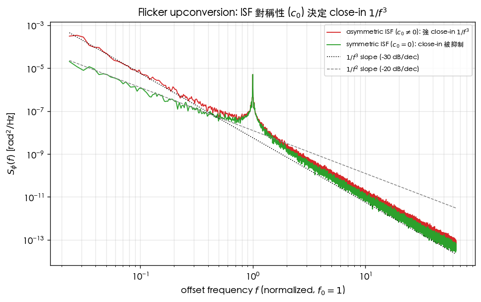
8. Simulation figure

9. How to read the figure

• Red line (asymmetric, $c_0\neq0$): in the close-in (low-offset) region a tall, steep curve appears, with slope near $-30$ dB/dec ($1/f^3$). The black dotted line is a pure $1/f^3$ slope reference; the red line hugs it.
• Green line (symmetric, $c_0=0$): clearly much lower in the close-in region, with a gentler slope (near $1/f^2$, gray dashed reference). $1/f^3$ is suppressed — visual proof that "waveform symmetry cuts close-in noise for free".
• The two lines converge at higher offsets: far from the carrier, the gap between $1/f^3$ and $1/f^2$ shrinks, because flicker noise itself is already weak at high frequency.
• Key point: the only difference between the two ISFs is $c_0$. The huge close-in gap between red and green is caused entirely by $c_0$. As $c_0\to0$, the red line collapses onto the green one.

10. Corresponding paper equations/figures

• Flicker noise source: [P1] Eq.(22), p.185, $\overline{i_{n,1/f}^2}=\overline{i_n^2}\cdot\omega_{1/f}/\Delta\omega$.
• $1/f^3$ close-in: [P1] Eq.(23), p.185; the prefactor $c_0^2$ is exactly this lab's switch.
• $1/f^3$ corner: [P1] Eq.(24), p.185, $\Delta\omega_{1/f^3}=\omega_{1/f}\,c_0^2/(2\Gamma_{rms}^2)\approx\omega_{1/f}(c_0/c_1)^2$.
• Concept-figure source: paper_001 Eqs (23),(24); the symmetry argument of paper_002. Corresponding site figure flicker_upconversion_symmetric_vs_asymmetric.png. For the geometric meaning of $c_0$ see also symmetric_vs_asymmetric_isf_c0.png in lab_05.

11. Limitations and approximations

• Pedagogical toy model, not transistor-level: the two ISFs (cos, cos+0.5) are teaching toys, not extracted from real circuits. The +0.5 is an artificially set $c_0$, purely for a controlled comparison.
• Normalized units: $f_0=1$, $q_{max}=1$, k_flicker on an arbitrary scale — no absolute dBc/Hz. The relative shape of the curves (slopes, red–green gap) is the teaching point.
• Flicker generation is approximate: flicker_noise uses frequency-domain $1/\sqrt f$ shaping and relies on f_low to tame the divergent DC bin; accuracy at very low frequency is limited by f_low and the total record length.
• Stationary-noise assumption: real flicker upconversion also involves cyclostationary modulation (the device leaks noise only while conducting); the full treatment uses $\Gamma_{eff}=\Gamma\cdot\alpha$ (see effective_isf); this lab demonstrates only the $c_0$ mechanism.
• Welch low-frequency scatter: the close-in region has few points and large statistical scatter; the plot shows only the trustworthy segment $f>0.02$.

Key takeaways

• Device $1/f$ noise is concentrated near DC; whether it upconverts into phase noise is determined by the ISF's DC component ($c_0/2$).
• $c_0\neq0$ → close-in $1/f^3$ ($-30$ dB/dec); $c_0=0$ → suppressed, falls back to $1/f^2$.
• The $1/f^3$ height is proportional to $c_0^2$; the corner $\propto c_0^2/\Gamma_{rms}^2$.
• Design lesson: making the waveform symmetric (suppressing $c_0$) is a free way to lower close-in phase noise.

Further reading

• Full theory derivation: flicker_noise_upconversion
• Fourier geometry of $c_0$: lab_05_fourier_isf
• Previous lab (white noise → 1/f²): lab_06_white_noise_phase_noise
• Use in design/theory: make the waveform symmetric (suppress $c_0$) to lower close-in $1/f^3$ → symmetry