β: This English translation is in beta — the Traditional-Chinese original is the authoritative version.

Lab 11 — Monte Carlo accumulated jitter — RJ is Gaussian, σ grows as √ΔN

Breadcrumb: Simulation labs › Noise & jitter › This page (Monte Carlo accumulated jitter). Upstream: oscillator_phase, lab_03; downstream: lab_12, lab_13.

This lab uses the most direct method — Monte Carlo (large-scale random sampling statistics) — to prove that the random jitter (RJ, Gaussian, unbounded) accumulated by a free-running (unlocked) oscillator has two key properties:

1. its distribution is Gaussian;
2. its standard deviation grows as the square root of the accumulated period count: $\sigma_{\Delta t}=\sigma_{edge}\sqrt{\Delta N}$.

This is the junction between the "statistical (time-domain) view" and the "spectral view", and it is the microscopic origin of [P2] Eq.(8), $\sigma_{\Delta t}=\kappa\sqrt{\Delta t}$.

Physical intuition (conclusion first): every period, noise pushes the oscillator's edge (zero-crossing/transition instant) by an independent small amount, mean 0, standard deviation $\sigma_{edge}$. Phase has no restoring force (see oscillator_phase), so these small pushes are never pulled back — they simply accumulate. This is a one-dimensional random walk. After $\Delta N$ steps, a random walk's position still has mean 0, but its variance is $\Delta N$ times the single-step variance, so the standard deviation grows as $\sqrt{\Delta N}$. And a sum of independent small increments tends to Gaussian by the central limit theorem.

1. Learning objectives

• Use Monte Carlo to directly "see" the Gaussian distribution of accumulated jitter.
• Verify the random-walk law $\sigma_{\Delta t}=\sigma_{edge}\sqrt{\Delta N}$: a $4\times$ increase in $\Delta N$ gives only a $2\times$ increase in $\sigma$.
• Link this time-domain result to [P2] Eq.(8), $\sigma_{\Delta t}=\kappa\sqrt{\Delta t}$ ($\kappa$ a proportionality constant).
• Understand why phase/jitter accumulates — because phase has no restoring force (unlike amplitude).

2. Mathematical model

Per-period increment. The edge-timing error of the $k$-th period is an i.i.d. Gaussian increment:

$$\delta_k\sim\mathcal{N}(0,\;\sigma_{edge}^2).$$

Accumulated jitter = sum of increments (random walk). After accumulating $\Delta N$ periods, the timing error relative to the ideal edge is:

$$\Delta t_{\Delta N}=\sum_{k=1}^{\Delta N}\delta_k .$$

Statistical properties (step by step). The increments are independent with zero mean:

$$\begin{aligned} \mathbb{E}[\Delta t_{\Delta N}]&=\sum_{k=1}^{\Delta N}\mathbb{E}[\delta_k]=0,\\ \operatorname{Var}[\Delta t_{\Delta N}]&=\sum_{k=1}^{\Delta N}\operatorname{Var}[\delta_k]=\Delta N\cdot\sigma_{edge}^2,\\ \sigma_{\Delta t}&=\sqrt{\operatorname{Var}}=\sigma_{edge}\sqrt{\Delta N}. \end{aligned}$$

• Why variances add: the variance of a sum of independent random variables equals the sum of the individual variances (zero covariance). This is the entire origin of the "$\sqrt{\Delta N}$".
• Why it's Gaussian: a sum of $\Delta N$ independent increments tends to Gaussian by the central limit theorem (and since each increment is already Gaussian, the sum is exactly Gaussian).
• Dimension check: $\sigma_{edge}$ is in s, $\sqrt{\Delta N}$ is dimensionless ($\Delta N$ is a period count), so $\sigma_{\Delta t}$ is in s ✓.

Linking to [P2] Eq.(8). Convert the accumulated period count into accumulated time $\Delta t=\Delta N\cdot T=\Delta N/f_0$:

$$\sigma_{\Delta t}=\sigma_{edge}\sqrt{\Delta N}=\sigma_{edge}\sqrt{f_0\,\Delta t}=\underbrace{\big(\sigma_{edge}\sqrt{f_0}\big)}_{\kappa}\sqrt{\Delta t},$$

i.e., [P2] Eq.(8), p.792, $\sigma_{\Delta t}=\kappa\sqrt{\Delta t}$, with $\kappa=\sigma_{edge}\sqrt{f_0}$.

• Dimension check ($\kappa$): $[\text{s}]\cdot[\text{Hz}]^{1/2}=[\text{s}]\cdot[\text{s}^{-1/2}]=[\text{s}^{1/2}]$, consistent with the unit $\sqrt{s}$ given for $\kappa$ in the canonical symbol table ✓.

3. Block diagram

4. Core Python code

Verbatim excerpt from main() in simulations/lab_11_monte_carlo_jitter.py: for each accumulation length lag (=$\Delta N$), draw n_trials × lag independent Gaussian increments, sum along the period axis to get the accumulated error acc, measure its std, then overlay the theoretical Gaussian.

f0 = 5e9
sigma_edge = 50e-15  # 50 fs per period
n_trials = 200000
lags = [25, 100, 400]  # number of periods accumulated

for lag, c in zip(lags, colors):
    incr = sigma_edge * RNG.standard_normal((n_trials, lag))
    acc = incr.sum(axis=1)  # accumulated timing error after `lag` periods
    sigma_meas = np.std(acc)
    sigma_theory = sigma_edge * np.sqrt(lag)
    # histogram (in fs)
    ax.hist(acc / 1e-15, bins=120, density=True, alpha=0.35, color=c,
            label=fr"$\Delta N$={lag}: 量得 $\sigma$={sigma_meas/1e-15:.0f} fs "
                  fr"(理論 {sigma_theory/1e-15:.0f} fs)")
    # gaussian overlay
    xx = np.linspace(acc.min(), acc.max(), 300)
    g = np.exp(-xx ** 2 / (2 * sigma_theory ** 2)) / (sigma_theory * np.sqrt(2 * np.pi))
    ax.plot(xx / 1e-15, g * 1e-15, color=c, lw=1.6)

• incr.sum(axis=1) sums lag independent increments — a one-dimensional random walk.
• sigma_meas = np.std(acc) (measured) converges digit by digit to sigma_theory = sigma_edge*np.sqrt(lag) (theoretical), because n_trials=200000 is large enough.
• The Gaussian overlay g uses the theoretical $\sigma$; its match to the histogram is the proof that the distribution is Gaussian.

Expected numbers ($\sigma_{edge}=50$ fs): $\Delta N=25\to250$ fs, $\Delta N=100\to500$ fs, $\Delta N=400\to1000$ fs (each $\times4$ step in $\Delta N$ gives $\times2$ in $\sigma$).

5. Full script path

simulations/lab_11_monte_carlo_jitter.py (dependency: savefig from simulations/common/plot_utils.py. Everything else uses numpy/matplotlib.)

Run with: python scripts/run_all_sims.py.

6. Parameter table

Parameter	Variable	Value	Notes
Oscillation frequency	f0	$5\times10^{9}$ Hz	5 GHz (used for the $\Delta N\leftrightarrow\Delta t$ conversion)
Per-period jitter	sigma_edge	$50\times10^{-15}$ s	rms increment per edge per period (50 fs)
Monte Carlo trials	n_trials	$200000$	trials per $\Delta N$
Accumulated period counts	lags	$\{25,100,400\}$	$\Delta N$, in a $\times4$ geometric progression
Histogram bins	—	$120$	density histogram
Random seed	RNG	default_rng(11)	reproducible results

7. Units table

Quantity	Symbol	Unit	Value in this lab
Per-period increment	$\delta_k,\ \sigma_{edge}$	s	$\sigma_{edge}=50$ fs
Accumulated period count	$\Delta N$	— (count)	25 / 100 / 400
Accumulated jitter	$\Delta t,\ \sigma_{\Delta t}$	s	250 / 500 / 1000 fs
Accumulated time	$\Delta t=\Delta N/f_0$	s	time spanned by $\Delta N$ periods
Proportionality constant	$\kappa=\sigma_{edge}\sqrt{f_0}$	$\sqrt{s}$	$\approx3.5\times10^{-12}\,\sqrt{s}$
Probability density	—	1/s (1/fs on the plot)	Gaussian curve

8. Simulation plot

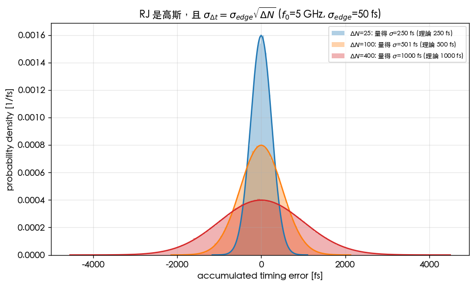
9. How to read the plot

• Three bell curves (blue/orange/red for $\Delta N=25/100/400$): the histogram (translucent) and the theoretical Gaussian curve (solid line) overlap almost perfectly — this is direct evidence that "RJ is Gaussian".
• Wider means longer accumulation: as $\Delta N$ grows, the bell gets shorter and wider. Note the width ($\sigma$) grows only as $\sqrt{\Delta N}$: from $25\to100$ ($\times4$), $\sigma$ goes from 250 fs to 500 fs (only $\times2$); from $100\to400$ (another $\times4$), 500 fs becomes 1000 fs (another $\times2$).
• "Measured σ vs. theoretical" in the legend: the two numbers are nearly identical, quantitatively verifying $\sigma_{\Delta t}=\sigma_{edge}\sqrt{\Delta N}$.
• How to use it: this explains why a free-running oscillator's long-term stability cannot be described by "per-period jitter" alone — jitter grows with observation time. Stopping the accumulation requires a PLL/CDR to lock the phase back to a reference (see lab_13).

10. Corresponding paper equations/figures

• Core correspondence: [P2] A. Hajimiri, S. Limotyrakis, and T. H. Lee, "Jitter and Phase Noise in Ring Oscillators," IEEE JSSC, 34(6), 1999, Eq.(8), p.792: $\sigma_{\Delta t}=\kappa\sqrt{\Delta t}$. This lab proves its microscopic origin is a random walk of per-edge Gaussian increments, and derives $\kappa=\sigma_{edge}\sqrt{f_0}$.
• Spec Section 10.2, "period / cycle-to-cycle jitter kernels": accumulated jitter "has no differencing (low-frequency dominated)", corresponding to the pure accumulation here (no high-pass differencing kernel).
• Phase has no restoring force (hence accumulates): [P1]'s LTV phase model (canonical formula 11), consistent with the geometry in oscillator_phase.
• Corresponds to site figure monte_carlo_jitter_histogram.png; echoes the time-domain accumulation plot ring_oscillator_timing_noise_accumulation.png in lab_03.

11. Limitations and approximations

• This is a pedagogical toy model, not transistor-level: we directly assume an independent Gaussian increment $\sigma_{edge}$ per period, without deriving its numerical value from ISF + device noise (that requires [P2]'s $\kappa$/FOM formulas, canonical formulas 22–23, verified verbatim against [P2] Eq.(8)/(12) p.792-793, Eq.(16) p.794, Eq.(23) p.796).
• Pure RJ, independent increments: assumes period-to-period noise is uncorrelated (white at the period scale). Real $1/f$ (flicker) noise introduces correlated increments, causing long-term accumulation to deviate from pure $\sqrt{\Delta N}$ (close-in $1/f^3$, see lab_07).
• Only covers accumulated/long-term jitter: period jitter (single-period deviation) and cycle-to-cycle jitter (adjacent difference) are the first/second-order differences of phase and are outside the scope of this plot (spec Section 10.2).
• Gaussian, unbounded: RJ is described by $\sigma$ with tails extending to infinity — this is exactly why SerDes BER is always $>0$ (see lab_12). Deterministic jitter (DJ, bounded) is outside this model.
• Finite-sample error: the small difference between sigma_meas and sigma_theory comes from finite n_trials; increasing it improves convergence.

Key takeaways

• Accumulated jitter is a random walk of per-edge Gaussian increments: mean 0, variance $\propto\Delta N$, Gaussian distribution.
• $\sigma_{\Delta t}=\sigma_{edge}\sqrt{\Delta N}$: a $4\times$ increase in $\Delta N$ gives only a $2\times$ increase in $\sigma$.
• Converting to time gives [P2] Eq.(8), $\sigma_{\Delta t}=\kappa\sqrt{\Delta t}$, with $\kappa=\sigma_{edge}\sqrt{f_0}$.
• No restoring force on phase → jitter accumulates → poor free-running long-term stability → needs a PLL/CDR to lock it back.

Further reading

• Why phase has no restoring force: oscillator_phase
• Time-domain accumulation plot for the ring oscillator: lab_03_ring_oscillator_toy_model
• How a PLL/CDR stops the accumulation: lab_13_pll_cdr_transfer
• RJ → SerDes BER: lab_12_serdes_eye_ber
• Applied to design/theory: how accumulated jitter eats into the SerDes timing budget → serdes_clocking_connection