β: This English translation is in beta — the Traditional-Chinese original is the authoritative version.

Phase Noise → Jitter

Prerequisites: white_noise_to_phase_noise · stochastic_noise_basics | Next: serdes_clocking_connection

This page answers the question engineers ask most often: you are handed a phase-noise plot ($\mathcal{L}(f)$, dBc/Hz) — how do you turn it into a single time-domain number, the rms jitter $\sigma_t$ (fs)? This is the bridge between the frequency domain (the language of communications/RF) and the time domain (the language of digital/SerDes).

The full chain is four steps:

$$\mathcal{L}(f)\ \xrightarrow{\ \times2,\ \text{de-dB}\ }\ S_\phi(f)\ \xrightarrow{\ \int_{f_1}^{f_2}\ }\ \sigma_\phi^2\ \xrightarrow{\ \sqrt{\ }\ }\ \sigma_\phi\ \xrightarrow{\ \div(2\pi f_0)\ }\ \sigma_t.$$

We take each step apart, carrying units and a dimension check throughout, and finish with canonical Example C (5 GHz, $-100$ dBc/Hz @ 1 MHz, 1/f² slope, 1→100 MHz) to obtain $\sigma_t=447.9$ fs.

Physical intuition (conclusion first): the phase error $\Delta\phi$ is "how far the clock hand has strayed in angle"; divide that angle by the angular velocity $2\pi f_0$ and you get "how far the hand has strayed in time," $\Delta t$. The phase-noise plot tells you how much phase power density sits at each offset frequency; adding it all up (integrating) gives the total phase variance; the square root is the rms phase; dividing by $2\pi f_0$ gives the rms timing jitter. The whole plot is compressed into one fs number.

Step 1: why a phase error becomes a timing error

An ideal oscillation $\cos(2\pi f_0 t)$ becomes $\cos(2\pi f_0 t+\Delta\phi)$ once excess phase is added. Factor the phase term out and look at where the zero crossing lands:

$$2\pi f_0 t+\Delta\phi=2\pi f_0\Big(t+\underbrace{\frac{\Delta\phi}{2\pi f_0}}_{=\ \Delta t}\Big).$$

In other words, an extra phase $\Delta\phi$ is equivalent to shifting the entire waveform along the time axis by $\Delta t$ (spec §3, Eq. 17):

$$\boxed{\ \Delta t=\frac{\Delta\phi}{2\pi f_0}\ }$$

• Physics used: the conversion rate between phase and time is the angular frequency $\omega_0=2\pi f_0$ (rad/s).
• Dimension check: $[\text{rad}]/[\text{rad/s}]=[\text{s}]$ ✓. Note the denominator is $2\pi f_0$ (rad/s), not $f_0$ (Hz) — dropping this $2\pi$ is the most common mistake.
• Why it is reasonable: at small phase ($\Delta\phi\ll1$ rad), phase offset and edge-time offset are linear and one-to-one. Timing jitter is the time error of the zero crossing, so it equals $\Delta\phi/(2\pi f_0)$.
• Feel: at 5 GHz, $\Delta\phi=1$ mrad $\Rightarrow\Delta t=31.8$ fs (see numerical_feeling Example 1).

Step 2: converting dBc/Hz to linear and recovering the phase PSD

The vertical axis of a phase-noise plot is $\mathcal{L}(f)$, the SSB phase noise (single-sideband phase noise), in dBc/Hz — meaning "at offset $f$, within a 1 Hz bandwidth, how many dB below the carrier the single-sideband noise power sits" (dBc = dB relative to carrier).

de-dB (from dB back to linear): dBc/Hz is $10\log_{10}(\cdot)$, so

$$\mathcal{L}_{\text{lin}}(f)=10^{\mathcal{L}(f)/10}\quad[\text{1/Hz}].$$

Then connect to the phase PSD: under the small-angle approximation, the SSB phase noise relates to the single-sided phase PSD as (spec §3, Eq. 16):

$$\boxed{\ \mathcal{L}(f)\approx\tfrac12\,S_\phi(f)\ }\quad\Longrightarrow\quad S_\phi(f)=2\cdot10^{\mathcal{L}(f)/10}\ [\text{rad}^2/\text{Hz}].$$

• Units: $S_\phi$ is $\text{rad}^2/\text{Hz}$ (the density of phase variance). $\mathcal{L}_{\text{lin}}$ itself is dimensionless per Hz; after multiplying by 2 it is read as $\text{rad}^2/\text{Hz}$.
• Where this $\frac12$ comes from: phase-modulation power splits evenly between the upper and lower sidebands, and $\mathcal{L}$ counts only one side, so it is half of $S_\phi$. This is exactly the bookkeeping convention discussed in the spec §3 "factor-of-2 teaching note"; for jitter integrals this site always uses $S_\phi=2\mathcal{L}_{\text{lin}}$. For a deeper discussion see white_noise_to_phase_noise.

Step-by-step derivation: $\mathcal{L}\approx\tfrac12 S_\phi$ comes from small-angle (narrowband) PM

That $\frac12$ above is not pulled out of thin air; it is a direct consequence of narrowband phase modulation (PM with a very small phase swing). We derive it step by step and make "one sideband's power $=(\phi_p/2)^2$" explicit.

Step 1: write a carrier phase-modulated by a single tone. Let the phase be modulated at a single frequency $\omega_m$ (offset angular frequency) with a small amplitude $\phi_p$ (peak phase, the peak of the phase swing, rad):

$$v(t)=\cos\big(\omega_0 t+\phi(t)\big),\qquad \phi(t)=\phi_p\sin\omega_m t,\quad \phi_p\ll 1\ \text{rad}.$$

• Physics used: this is Step 1's excess phase $\Delta\phi$ replaced by a phase that swings sinusoidally in time; $\phi_p$ is its amplitude.
• Units: $\phi_p$ and $\phi(t)$ are both rad; $\omega_0,\omega_m$ are both rad/s.

Step 2: expand the phase modulation with a trig identity. Use the angle-sum formula $\cos(A+B)=\cos A\cos B-\sin A\sin B$ with $A=\omega_0 t$, $B=\phi(t)$:

$$v(t)=\cos\omega_0 t\,\cos\!\big(\phi_p\sin\omega_m t\big)-\sin\omega_0 t\,\sin\!\big(\phi_p\sin\omega_m t\big).$$

Step 3: the small-angle approximation (this is all "small-angle" means). Because $\phi_p\ll1$:

$$\cos\!\big(\phi_p\sin\omega_m t\big)\approx 1,\qquad \sin\!\big(\phi_p\sin\omega_m t\big)\approx \phi_p\sin\omega_m t.$$

• Math used: Taylor expansions $\cos x\approx1-x^2/2$, $\sin x\approx x$, keeping first order only ($x=\phi_p\sin\omega_m t$, whose $x^2$ is $O(\phi_p^2)$ and can be dropped). This is exactly the small-amplitude limit of the Bessel expansion $J_0\approx1,\ J_1\approx\phi_p/2$.

Substituting back:

$$v(t)\approx\cos\omega_0 t-\phi_p\sin\omega_0 t\,\sin\omega_m t.$$

Step 4: split $\sin\times\sin$ into the two sidebands. Use the product-to-sum identity $\sin\alpha\sin\beta=\tfrac12[\cos(\alpha-\beta)-\cos(\alpha+\beta)]$ with $\alpha=\omega_0 t$, $\beta=\omega_m t$:

$$\begin{aligned} v(t)&\approx\cos\omega_0 t-\frac{\phi_p}{2}\Big[\cos(\omega_0-\omega_m)t-\cos(\omega_0+\omega_m)t\Big]\\ &=\underbrace{\cos\omega_0 t}_{\text{carrier}}-\underbrace{\frac{\phi_p}{2}\cos(\omega_0-\omega_m)t}_{\text{lower sideband}}+\underbrace{\frac{\phi_p}{2}\cos(\omega_0+\omega_m)t}_{\text{upper sideband}}. \end{aligned}$$

• Physical meaning: phase modulation grows a symmetric pair of sidebands next to the carrier, at $\omega_0\pm\omega_m$, each with amplitude $\phi_p/2$. This is the time-domain origin of the "carrier smeared into a skirt" picture of [P1] Fig. 8.

Step 5: each sideband's relative power. The carrier has amplitude $1$, power $\propto 1$ (taking $\tfrac12\cdot1^2$); a single sideband has amplitude $\phi_p/2$, power $\propto(\phi_p/2)^2$. So the single-sideband-to-carrier power ratio is

$$\frac{P_{\text{1 sideband}}}{P_{\text{carrier}}}=\frac{\tfrac12(\phi_p/2)^2}{\tfrac12(1)^2}=\Big(\frac{\phi_p}{2}\Big)^2=\frac{\phi_p^2}{4}.$$

• Dimension check: a power ratio is dimensionless ✓; $\phi_p$ (rad) squared is read as $\text{rad}^2$ in the "phase power" context.

Step 6: connect it to $S_\phi$. For $\phi(t)=\phi_p\sin\omega_m t$, the mean square (variance) of the phase is

$$\langle\phi^2(t)\rangle=\phi_p^2\langle\sin^2\omega_m t\rangle=\frac{\phi_p^2}{2}.$$

All of this single tone's phase power $\phi_p^2/2$ is concentrated in the one spectral line at $\omega_m$; reading it as "the single-sided phase-PSD strength at $\omega_m$" gives $S_\phi(\omega_m)=\phi_p^2/2$ (per-Hz, taken as the weight of one line).

Step 7: divide the two, and the $\frac12$ appears. $\mathcal{L}$ (SSB) = single-sideband power ratio $=\phi_p^2/4$; $S_\phi=\phi_p^2/2$. So

$$\boxed{\ \mathcal{L}=\frac{\phi_p^2/4}{1}=\frac12\cdot\frac{\phi_p^2}{2}=\frac12 S_\phi\ }$$

• One-sentence summary: $\mathcal{L}$ counts one sideband (power $(\phi_p/2)^2=\phi_p^2/4$), while $S_\phi$ is the total phase power density ($\phi_p^2/2$, i.e. the two sidebands combined). One side ÷ total $=\tfrac12$ — that is the entire origin of the factor-of-$\tfrac12$.
• Failure condition: once $\phi_p$ is no longer $\ll1$, the higher-order Bessel terms of Step 3 ($J_2,J_3,\dots$) grow additional sidebands and $\mathcal{L}=\tfrac12 S_\phi$ no longer holds — at large phase the carrier also "loses power" to the higher-order sidebands.
• Small-angle condition: $\mathcal{L}\approx\frac12 S_\phi$ holds only for $\sigma_\phi\ll1$ rad (Bessel expansion kept to first order). Here $\sigma_\phi=14$ mrad $\ll1$, OK.
• Canonical numbers: at 1 MHz, $\mathcal{L}=-100$ dBc/Hz: $\mathcal{L}_{\text{lin}}=10^{-100/10}=10^{-10}$; $S_\phi(1\text{MHz})=2\times10^{-10}\ \text{rad}^2/\text{Hz}$.

Step 3: why integrating the phase PSD gives the variance

This step is pure Parseval / Wiener–Khinchin: integrate the PSD over frequency to obtain the time-domain variance (spec §3, Eq. 18):

$$\boxed{\ \sigma_\phi^2=\int_{f_1}^{f_2}S_\phi(f)\,df\ }$$

• Math used: $S_\phi(f)$ is "phase power per unit bandwidth"; summing (integrating) it over the offset band of interest $[f_1,f_2]$ gives the total phase power = the variance $\sigma_\phi^2$. This is the same move as integrating the current PSD into $\overline{i_n^2}$ in Section 3 of stochastic_noise_basics.
• Dimension check: $(\text{rad}^2/\text{Hz})\times\text{Hz}=\text{rad}^2$ ✓.
• Why the integration band $[f_1,f_2]$ matters: the phase PSD at low offset is typically 1/f² (or even 1/f³), so the integral is dominated by the lower limit $f_1$. Moving $f_1$ by one decade can change the jitter by several times. So a reported jitter number must state its integration bandwidth, otherwise it is meaningless.
  • Upper limit $f_2$: physically set by the system bandwidth (for SerDes, the PLL loop bandwidth or Nyquist).
  • Lower limit $f_1$: for an open-loop oscillator the integral diverges toward DC (random walk); in practice it is set by the measurement time or by the frequency at which a PLL "holds" the phase.
• Small-angle approximation ($\sin\Delta\phi\approx\Delta\phi$): approximating the phase-modulation power as $\sigma_\phi^2$ likewise requires $\sigma_\phi\ll1$ rad.

The closed-form 1/f² integral (the core of this example)

Anchor the 1/f² shape from Step 2 at $f_{ref}=1$ MHz:

$$S_\phi(f)=S_\phi(f_{ref})\Big(\frac{f_{ref}}{f}\Big)^2=2\times10^{-10}\Big(\frac{10^6}{f}\Big)^2.$$

Substitute into the integral (note $\int f^{-2}df=-1/f$):

$$\begin{aligned} \sigma_\phi^2&=2\times10^{-10}\,(10^6)^2\int_{10^6}^{10^8}\frac{df}{f^2} =2\times10^{2}\Big(\frac{1}{10^6}-\frac{1}{10^8}\Big)\\ &=200\times(10^{-6}-10^{-8})=200\times9.9\times10^{-7}=1.98\times10^{-4}\ \text{rad}^2. \end{aligned}$$

Take the square root:

$$\sigma_\phi=\sqrt{1.98\times10^{-4}}=1.407\times10^{-2}\ \text{rad}=14.07\ \text{mrad}.$$

• Feel check: inside the parentheses $10^{-6}\gg10^{-8}$, so the "$1/f_1$" term dominates — confirming again that the lower limit dominates. Raising $f_2$ from 100 MHz to 1 GHz barely changes the answer; lowering $f_1$ from 1 MHz to 100 kHz blows the jitter up by $\sqrt{10}\approx3.2\times$.

Step 4: phase variance → rms jitter

Apply Step 1's $\Delta t=\Delta\phi/(2\pi f_0)$ to the rms quantities (spec §3, Eq. 19):

$$\boxed{\ \sigma_t=\frac{\sigma_\phi}{2\pi f_0}=\frac{1}{2\pi f_0}\sqrt{\int_{f_1}^{f_2}S_\phi(f)\,df}\ }$$

Substituting this example ($f_0=5$ GHz, $\sigma_\phi=1.407\times10^{-2}$ rad):

$$\sigma_t=\frac{1.407\times10^{-2}\ \text{rad}}{2\pi\times5\times10^{9}\ \text{Hz}} =\frac{1.407\times10^{-2}}{3.1416\times10^{10}}\ \text{s} =4.479\times10^{-13}\ \text{s}=447.9\ \text{fs}.$$

• Dimension check: $[\text{rad}]/[\text{rad/s}]=[\text{s}]$ ✓.
• This is canonical Example C (spec §8): 5 GHz, $-100$ dBc/Hz @ 1 MHz, 1/f², integrated 1→100 MHz $\Rightarrow\sigma_\phi=14.07$ mrad, $\sigma_t=447.9$ fs.
• Scaling feel: 10 dB better phase noise ($\mathcal{L}=-110$) $\Rightarrow S_\phi$ 10× smaller $\Rightarrow\sigma_t$ smaller by $\sqrt{10}\approx3.2\times$ $\to\sim142$ fs. 20 dB better ($-120$) $\Rightarrow$ 10× smaller $\to\sim45$ fs (see the reference points in numerical_feeling).

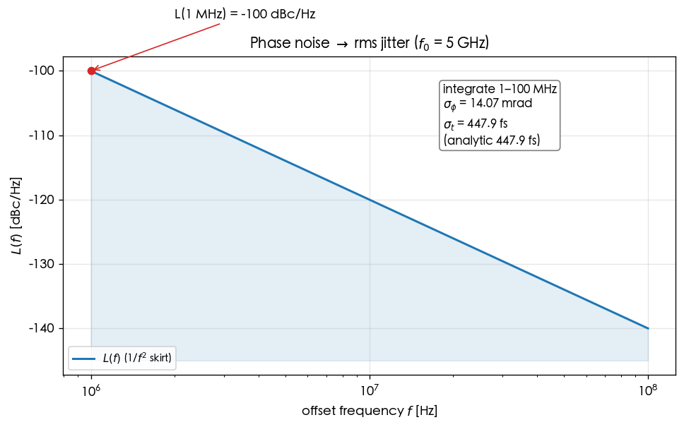
The figure above (simulations/lab_08_jitter_integration.py) plots the 1/f² skirt at $-100$ dBc/Hz @ 1 MHz and how the cumulative integral converges to 447.9 fs with bandwidth; the numerical integration matches the hand-computed analytic result above exactly. This is a toy / analytic demo (single 1/f² source, small-angle approximation), not transistor-level.

One-line verification (using the built-in functions)

import numpy as np
from simulations.common.noise_utils import leeson_one_over_f2, integrate_rms_jitter

f = np.logspace(6, 8, 4000)                              # 1 MHz -> 100 MHz
L = leeson_one_over_f2(f, L_ref_dbc=-100, f_ref=1e6)     # 1/f^2 skirt
sigma_t, sigma_phi = integrate_rms_jitter(f, L, f0=5e9, fmin=1e6, fmax=100e6)
print(sigma_phi*1e3, "mrad ;", sigma_t*1e15, "fs")       # -> 14.07 mrad ; 447.9 fs

The four "dialects" of jitter (using the notation page's table)

The same word "jitter" can refer to entirely different measured quantities. The table below follows the definitions of notation (spec §2):

Name	Definition	Intuition	Relation to phase noise
random jitter (RJ)	Gaussian, unbounded, described by $\sigma$	wander from random kicks	exactly the $\sigma_t$ integrated above; SerDes BER uses it to estimate eye closure
period jitter	$T_k-T$ (a single period relative to nominal)	how long/short this one beat is	integrate $S_\phi$ after applying a $\sin^2(\pi f/f_0)$-type high-pass weight
cycle-to-cycle jitter	$T_{k+1}-T_k$ (difference of adjacent periods)	how fast the beat changes beat to beat	differences adjacent periods; even stronger high-pass weighting, least affected by close-in
accumulated / long-term jitter	edge error over separation $\Delta t$, $\sigma_{\Delta t}=\kappa\sqrt{\Delta t}$	an open-loop oscillator drifts further the longer it runs	random walk; corresponds to integrating 1/f² down to very low offset ([P2] Eq.(8))

• Why the distinction matters: period / cycle-to-cycle jitter apply a high-pass weight to $S_\phi$ (differencing suppresses low frequencies and amplifies high ones), so they are not dominated by close-in 1/f²; whereas the random / integrated jitter computed above (the absolute zero-crossing time error) is dominated by the lower limit. When reporting a number, say which kind it is, or the figures can differ by orders of magnitude.
• accumulated jitter: a free-running oscillator has no absolute time reference; its phase is a random walk, $\sigma_{\Delta t}=\kappa\sqrt{\Delta t}$ ([P2] Eq.(8), p.792, claim C6). For ring details see [P2] and serdes_clocking_connection.

Weighting kernels for period / cycle-to-cycle / accumulated jitter (step-by-step derivation)

The "high-pass weighting" in the table above is not hand-waving; it has exact kernels. Key idea: the different kinds of jitter are different "differences" of the same phase process $\phi(t)$, and a time-domain difference is, in the frequency domain, multiplication by a transfer function. We derive the kernels step by step.

Step 1: write each edge's time error as a sample of the phase. The $k$-th edge nominally lands at $t_k=kT$; its time error is the phase at that instant divided by the angular velocity (reusing Step 1's $\Delta t=\Delta\phi/(2\pi f_0)$):

$$\Delta t_k=\frac{\phi(kT)}{2\pi f_0}.$$

Step 2: three jitters = three differences. By definition (spec §2):

$$\begin{aligned} \text{period jitter:}\quad &J^{\text{per}}_k=\Delta t_{k+1}-\Delta t_k=\frac{\phi((k{+}1)T)-\phi(kT)}{2\pi f_0}\quad(\text{first difference of the phase}),\\ \text{cycle-to-cycle:}\quad &J^{\text{c2c}}_k=J^{\text{per}}_{k+1}-J^{\text{per}}_k\quad(\text{second difference of the phase}),\\ \text{accumulated:}\quad &\Delta t_k=\frac{\phi(kT)}{2\pi f_0}\quad(\text{no differencing; the phase itself}). \end{aligned}$$

Step 3: differencing in the frequency domain = multiplying by $(1-e^{-j2\pi fT})$. For a frequency component $\phi(t)\propto e^{j2\pi ft}$, a delay of one period $T$ is multiplication by $e^{-j2\pi fT}$. So the frequency response of the first-difference operator "now minus one period ago" is

$$H_{\text{per}}(f)=1-e^{-j2\pi fT},\qquad \lvert H_{\text{per}}(f)\rvert^2=\big\lvert 1-e^{-j2\pi fT}\big\rvert^2=4\sin^2(\pi fT).$$

• Algebraic expansion: $\lvert 1-e^{-j\theta}\rvert^2=(1-\cos\theta)^2+\sin^2\theta=2-2\cos\theta=4\sin^2(\theta/2)$; substituting $\theta=2\pi fT$ gives $4\sin^2(\pi fT)$.
• Why it is high-pass: as $f\to0$, $\sin^2(\pi fT)\approx(\pi fT)^2\to0$ — low frequencies get crushed; the maximum of $4$ occurs at $f=f_0/2=1/(2T)$. This is the mathematical reason period jitter is "not dominated by close-in 1/f²".

Step 4: put the kernel into the phase-variance integral. Multiply the phase-variance density by $\lvert H\rvert^2$, integrate, then divide by $(2\pi f_0)^2$ to convert to time (spec §10.2, period/cycle-to-cycle jitter kernels):

$$\sigma_{T}^2=\frac{1}{(2\pi f_0)^2}\int_0^{\infty}S_\phi(f)\,\big\lvert 1-e^{-j2\pi fT}\big\rvert^2\,df =\frac{1}{(2\pi f_0)^2}\int_0^{\infty}S_\phi(f)\,4\sin^2(\pi fT)\,df.$$

Cycle-to-cycle takes one more difference, so the kernel is squared once more (a second difference = the first-difference operator applied twice):

$$\sigma_{cc}^2=\frac{1}{(2\pi f_0)^2}\int_0^{\infty}S_\phi(f)\,\big\lvert 1-e^{-j2\pi fT}\big\rvert^4\,df =\frac{1}{(2\pi f_0)^2}\int_0^{\infty}S_\phi(f)\,16\sin^4(\pi fT)\,df.$$

Accumulated jitter has no differencing kernel (kernel $=1$), so it is dominated by low frequencies (the 1/f² integral diverges once carried to very low offset), which is precisely the frequency-domain counterpart of its $\sqrt{\Delta t}$ random-walk growth ([P2] Eq.(8), p.792; κ from Eq.(12), p.793).

• Dimension check: $S_\phi$ ($\text{rad}^2/\text{Hz}$) × dimensionless kernel × $\text{Hz}$ = $\text{rad}^2$; dividing by $(2\pi f_0)^2$ ($\text{rad}^2/\text{s}^2$) gives $\text{s}^2$ ✓, and the square root yields seconds.
• Three-line comparison: accumulated kernel $=1$ (low-frequency dominated); period kernel $\lvert1-e^{-j2\pi fT}\rvert^2$ (first-order high-pass); cycle-to-cycle kernel $\lvert1-e^{-j2\pi fT}\rvert^4$ (second-order high-pass, least sensitive to close-in).

Note (constant conventions): the expressions above use the "single-sided $S_\phi$, $\int_0^\infty$" convention; with a double-sided PSD or a different SSB bookkeeping, the prefactor can differ by a factor of 2 — same root cause as the spec §3 factor-of-2 teaching note. For jitter this site always uses $S_\phi=2\mathcal{L}_{\text{lin}}$ with single-sided integration. For exact constants consult each reference's definitions.

Canonical numbers: period jitter integrated from $S_\phi$

Continuing Example C: $f_0=5$ GHz ($T=200$ ps), $\mathcal{L}(1\text{MHz})=-100$ dBc/Hz, 1/f² slope. Find the period jitter $\sigma_T$ (integrate 1 MHz→100 MHz, the same band as Example C for comparison).

Insert the 1/f² shape from Step 3, $S_\phi(f)=2\times10^{-10}(10^6/f)^2$, into the period kernel. First check the kernel's size over this band: $T=2\times10^{-10}$ s; $\pi fT$ at $f=10^6$ is $\pi\times10^6\times2\times10^{-10}=6.28\times10^{-4}\ll1$, and at $f=10^8$ it is $6.28\times10^{-2}\ll1$. So the small-angle form $\sin^2(\pi fT)\approx(\pi fT)^2$ applies over the whole band:

$$\big\lvert 1-e^{-j2\pi fT}\big\rvert^2\approx 4(\pi fT)^2=(2\pi fT)^2.$$

Substitute into the period integral:

$$\begin{aligned} \sigma_T^2&=\frac{1}{(2\pi f_0)^2}\int_{10^6}^{10^8}\!2\times10^{-10}\Big(\frac{10^6}{f}\Big)^2(2\pi fT)^2\,df\\ &=\frac{(2\pi T)^2}{(2\pi f_0)^2}\,2\times10^{-10}(10^6)^2\int_{10^6}^{10^8}\!df =T^4\cdot 2\times10^{-10}(10^6)^2\int_{10^6}^{10^8}\!df. \end{aligned}$$

Collect the constants: $(2\pi T)^2/(2\pi f_0)^2=T^2/f_0^2=T^2\cdot T^2=T^4$ (since $f_0=1/T$), and the two powers of $f$ cancel ($f^{-2}\cdot f^{2}=1$), so the integral becomes $\int_{10^6}^{10^8}df=9.9\times10^7$ Hz:

$$\begin{aligned} \sigma_T^2&=T^4\cdot 2\times10^{-10}\cdot(10^6)^2\cdot(9.9\times10^7)\\ &=(2\times10^{-10})^4\cdot 2\times10^{-10}\cdot10^{12}\cdot9.9\times10^7. \end{aligned}$$

Term by term: $T^4=(2\times10^{-10})^4=16\times10^{-40}=1.6\times10^{-39}$; $2\times10^{-10}\cdot10^{12}=2\times10^{2}$; multiplying by $9.9\times10^7$ gives $1.98\times10^{10}$. So

$$\sigma_T^2=1.6\times10^{-39}\times1.98\times10^{10}=3.17\times10^{-29}\ \text{s}^2 \;\Rightarrow\;\sigma_T=5.6\times10^{-15}\ \text{s}=5.6\ \text{fs}.$$

• Feel, side by side: same phase-noise plot, same integration band — the accumulated/RJ $\sigma_t=447.9$ fs (Example C, lower-limit dominated), yet the period jitter is only $\sim5.6$ fs — almost two orders of magnitude smaller! The reason is exactly the high-pass kernel $(2\pi fT)^2$ crushing the close-in end (the 1 MHz end, the main contributor to RJ); period jitter instead accumulates from the high-frequency end. This is the best possible teaching example of "always say which kind of jitter you are reporting."
• Dimension check: $T^4$ ($\text{s}^4$) $\times\,\text{(rad}^2/\text{Hz)}\times\text{Hz}\times f^{0}$ collapses to $\text{s}^2$ ✓.

import numpy as np
from simulations.common.noise_utils import phase_psd_to_l_dbc_per_hz  # noqa: F401
# period jitter: multiply S_phi by |1-e^{-j2πfT}|^2 = 4 sin^2(πfT), integrate, divide by (2πf0)^2
f  = np.logspace(6, 8, 200000)
f0 = 5e9; T = 1.0/f0
S_phi = 2e-10 * (1e6/f)**2                      # 1/f^2, reconstructed from -100 dBc/Hz @1MHz
kernel = np.abs(1 - np.exp(-1j*2*np.pi*f*T))**2 # = 4 sin^2(πfT) high-pass kernel
sigma_T = np.sqrt(np.trapezoid(S_phi*kernel, f)) / (2*np.pi*f0)
print(sigma_T*1e15, "fs period jitter")          # -> ~5.6 fs (far below the 447.9 fs RJ)

Validity and failure conditions

Condition	When it holds	When it fails
Small angle $\sigma_\phi\ll1$ rad	$\mathcal{L}\approx\frac12 S_\phi$; $\Delta t=\Delta\phi/(2\pi f_0)$ linear	large phase → full Bessel expansion needed, $\mathcal{L}\neq\frac12 S_\phi$
Finite, explicit integration band	$\sigma_t$ converges, reproducible	1/f² diverges when integrated to DC; a number without a stated band is meaningless
Single 1/f² shape (this example)	closed-form analytic result usable	real plots have 1/f³ + a flat floor; integrate piecewise or numerically
RJ is Gaussian	estimate BER from $\sigma$	with deterministic jitter (DJ) present, an RJ/DJ decomposition is required

Corresponding papers / formulas

• $\Delta t=\Delta\phi/(2\pi f_0)$, $\sigma_\phi^2=\int S_\phi df$, $\sigma_t=\sigma_\phi/(2\pi f_0)$, $\mathcal{L}\approx\frac12 S_\phi$: spec §3, Eqs. 16–19.
• accumulated jitter $\sigma_{\Delta t}=\kappa\sqrt{\Delta t}$: [P2] Eq.(8), p.792 (claim C6).
• the origin of phase noise itself (white noise → 1/f²): [P1] Eq.(21), p.185.
• figure: phase_noise_to_jitter_integration.png (lab_08), per spec §4.

Worked examples

The two problems below run the full chain and the weighting kernel once each. Format: problem → step-by-step substitution (with units) → result → dimension check → one-line Python verification (using simulations/common/).

Example C: phase noise plot → rms jitter (canonical, $-100$ dBc/Hz → 447.9 fs)

Problem: $f_0=5$ GHz, $\mathcal{L}(1\text{MHz})=-100$ dBc/Hz, 1/f² slope, integrate 1 MHz→100 MHz; find the rms (accumulated/RJ) jitter $\sigma_t$.

Step 1 (de-dB + recover $S_\phi$): $\mathcal{L}_{\text{lin}}=10^{-100/10}=10^{-10}$; $S_\phi(1\text{MHz})=2\mathcal{L}_{\text{lin}}=2\times10^{-10}\ \text{rad}^2/\text{Hz}$.

Step 2 (1/f² shape):

$$S_\phi(f)=2\times10^{-10}\Big(\frac{10^6}{f}\Big)^2.$$

Step 3 (integrate for the variance, $\int f^{-2}df=-1/f$):

$$\sigma_\phi^2=2\times10^{-10}(10^6)^2\!\int_{10^6}^{10^8}\!\frac{df}{f^2} =2\times10^{2}\Big(\frac{1}{10^6}-\frac{1}{10^8}\Big)=200\times9.9\times10^{-7}=1.98\times10^{-4}\ \text{rad}^2.$$ $$\sigma_\phi=\sqrt{1.98\times10^{-4}}=1.407\times10^{-2}\ \text{rad}=14.07\ \text{mrad}.$$

Step 4 (convert to time):

$$\sigma_t=\frac{\sigma_\phi}{2\pi f_0}=\frac{1.407\times10^{-2}}{2\pi\times5\times10^{9}}=4.479\times10^{-13}\ \text{s}=447.9\ \text{fs}.$$

• Result: $\sigma_\phi=14.07$ mrad, $\sigma_t=447.9$ fs.
• Dimension check: Step 3 $(\text{rad}^2/\text{Hz})\times\text{Hz}=\text{rad}^2$ ✓; Step 4 $[\text{rad}]/[\text{rad/s}]=[\text{s}]$ ✓.
• Feel: the integral is dominated by the lower limit $f_1=1$ MHz ($1/f_1\gg1/f_2$); always state the bandwidth when reporting jitter.

import numpy as np
from simulations.common.noise_utils import leeson_one_over_f2, integrate_rms_jitter
f = np.logspace(6, 8, 4000)                            # 1 MHz -> 100 MHz
L = leeson_one_over_f2(f, L_ref_dbc=-100, f_ref=1e6)   # 1/f^2 skirt
sigma_t, sigma_phi = integrate_rms_jitter(f, L, f0=5e9, fmin=1e6, fmax=100e6)
print(sigma_phi*1e3, "mrad ;", sigma_t*1e15, "fs")     # -> 14.07 mrad ; 447.9 fs

Example D: same L(f) → period jitter (apply the high-pass kernel $\lvert1-e^{-j2\pi fT}\rvert^2$)

Problem: same as Example C ($f_0=5$ GHz, $T=200$ ps, $-100$ dBc/Hz @ 1 MHz, 1/f², integrate 1→100 MHz), but now find the period jitter $\sigma_T$ and see how far it differs from Example C's RJ.

Step 1 (small-angle form of the kernel): over this band $\pi fT\le 6.28\times10^{-2}\ll1$, so $\lvert1-e^{-j2\pi fT}\rvert^2=4\sin^2(\pi fT)\approx(2\pi fT)^2$.

Step 2 (substitute into the period integral and cancel the powers): prefactor $T^2/f_0^2=T^4$, and $f^{-2}\cdot f^{2}=1$:

$$\sigma_T^2=T^4\cdot2\times10^{-10}(10^6)^2\!\int_{10^6}^{10^8}\!df =T^4\cdot2\times10^{2}\cdot(9.9\times10^7).$$

Step 3 (substitute $T=2\times10^{-10}$ s): $T^4=1.6\times10^{-39}\ \text{s}^4$; the remaining factor $=1.98\times10^{10}$ ($\text{rad}^2\cdot\text{Hz}$, which multiplied by $T^4$ gives $\text{s}^2$):

$$\sigma_T^2=1.6\times10^{-39}\times1.98\times10^{10}=3.17\times10^{-29}\ \text{s}^2 \;\Rightarrow\;\sigma_T=5.6\ \text{fs}.$$

• Result: $\sigma_T\approx5.6$ fs, about $1/80$ of Example C's RJ (447.9 fs).
• Dimension check: $T^4(\text{s}^4)\times(\text{rad}^2/\text{Hz})\times\text{Hz}$ collapses to $=\text{s}^2$ ✓.
• Physics: the first-difference period kernel $(2\pi fT)^2$ crushes the close-in region (RJ's main contributor); period jitter accumulates from the high-frequency end → same plot, different kind of jitter, numbers two orders of magnitude apart.

import numpy as np
f  = np.logspace(6, 8, 200000)
f0 = 5e9; T = 1.0/f0
S_phi  = 2e-10 * (1e6/f)**2                          # reconstructed from -100 dBc/Hz @1MHz
kernel = np.abs(1 - np.exp(-1j*2*np.pi*f*T))**2      # 4 sin^2(πfT) high-pass kernel
sigma_T = np.sqrt(np.trapezoid(S_phi*kernel, f)) / (2*np.pi*f0)
print(sigma_T*1e15, "fs period jitter")              # -> ~5.6 fs (<< 447.9 fs RJ)

Key takeaways

• The four-step chain: dBc/Hz $\xrightarrow{\times2,\text{de-dB}} S_\phi\xrightarrow{\int}\sigma_\phi^2 \xrightarrow{\sqrt{}}\sigma_\phi\xrightarrow{\div2\pi f_0}\sigma_t$.
• $\Delta t=\Delta\phi/(2\pi f_0)$: phase divided by angular velocity = time; the denominator is $2\pi f_0$ (rad/s) — do not drop the $2\pi$.
• $S_\phi=2\cdot10^{\mathcal{L}/10}$; $\mathcal{L}\approx\frac12 S_\phi$ holds only at small angle.
• The 1/f² jitter integral is dominated by the lower limit $f_1$ — always state the integration bandwidth when reporting jitter.
• Canonical Example C: 5 GHz, $-100$ dBc/Hz @ 1 MHz, 1/f², 1→100 MHz $\Rightarrow$ $\sigma_\phi=14.07$ mrad, $\sigma_t=447.9$ fs.
• Four kinds of jitter: RJ / period / cycle-to-cycle / accumulated — different weightings, different dominant bands.
• The root of $\mathcal{L}=\tfrac12 S_\phi$: small-angle PM grows symmetric sidebands; one sideband's power is $(\phi_p/2)^2=\phi_p^2/4$, the total phase power is $\phi_p^2/2$, and one side ÷ total $=\tfrac12$.
• Weighting kernels: accumulated kernel $=1$ (low-frequency dominated); period kernel $\lvert1-e^{-j2\pi fT}\rvert^2=4\sin^2(\pi fT)$ (first-order high-pass); cycle-to-cycle kernel $\lvert1-e^{-j2\pi fT}\rvert^4$ (second-order high-pass).
• Same $-100$ dBc/Hz plot: RJ $\sigma_t=447.9$ fs, but the period jitter is only $\sim5.6$ fs — the high-pass kernel crushes close-in.

Further reading

• The three must-do mental-math drills (including this example): numerical_feeling
• Prerequisite basics for noise PSD / Parseval / cyclostationary: stochastic_noise_basics
• The DSP view: phase = a random process shaped by ISF weighting + an integrator: dsp_view_of_phase_noise
• Where phase noise itself comes from (white noise → 1/f²): white_noise_to_phase_noise
• Jitter's connection to SerDes: serdes_clocking_connection