β: This English translation is in beta — the Traditional-Chinese original is the authoritative version.

Allan Variance: The Time-Domain Counterpart of Phase Noise

Prerequisites: psd_phase_noise_jitter · white_noise_to_phase_noise ｜ Next: serdes_clocking_connection

The previous pages all viewed oscillator imperfection from the frequency domain: jitter was written as SSB phase noise $\mathcal{L}(\Delta f)$ (in dBc/Hz) or as the phase PSD $S_\phi(f)$ (in $\text{rad}^2/\text{Hz}$), then integrated into an rms jitter $\sigma_t$ (see psd_phase_noise_jitter). That language is the natural one for RF/communication circuits. But the people who work on clocks, frequency standards, GPS, and atomic clocks speak another language: the Allan variance and its square root, the Allan deviation / ADEV $\sigma_y(\tau)$. This page answers:

• What does $\sigma_y(\tau)$ actually measure? Why is it defined as the mean square of the "difference between two adjacent gated frequency averages"?
• How does it convert to the familiar $S_\phi(f)$ and $\mathcal{L}(\Delta f)$?
• Why does each of the five power-law noise types trace a characteristic slope on the ADEV log–log plot, so that the slopes "read out the noise type at a glance"?
• Why does the clock community prefer ADEV over the ordinary sample variance of frequency?

Physical intuition (conclusion first): take a stopwatch (the oscillator under test) and compare it against a perfect clock; every $\tau$ seconds record "over this $\tau$-second gate, how much faster/slower was my average frequency than nominal", producing a string of fractional frequency deviations $\bar y_k$. The ordinary variance asks "how far are these $\bar y_k$ from their grand mean" — but for flicker ($1/f$) and random-walk noise, the grand mean simply does not exist (it keeps drifting the longer you collect data), so the ordinary variance grows and grows without converging. Allan's trick: do not compare against the grand mean — compare only against the neighboring gate — $\tfrac12\langle(\bar y_{k+1}-\bar y_k)^2\rangle$. The adjacent subtraction cancels out the "slow drift", so even for flicker/RW noise the result converges and can be measured repeatably as a stable number. The price: it becomes a function of $\tau$ — the gate length $\tau$ you choose sets the time scale at which you probe stability.

ADEV is "phase noise in the time domain": the same physics (the same $S_\phi(f)$), just viewed in a different coordinate. Below we connect the two sides step by step.

Step 1: the fractional frequency deviation $y(t)$ and its PSD $S_y(f)$

First, define the protagonist. Let the instantaneous phase of the signal under test be $\omega_0 t+\phi(t)$, where $\phi(t)$ is the excess phase (the random offset relative to the ideal linear phase, in rad). The instantaneous fractional frequency deviation (dimensionless) is defined as the time derivative of the phase deviation divided by the nominal angular frequency:

$$y(t)=\frac{1}{\omega_0}\frac{d\phi(t)}{dt}=\frac{1}{2\pi f_0}\,\dot\phi(t).$$

• Physical meaning: $y$ is "by what fraction the frequency right now exceeds the nominal frequency". $y=10^{-9}$ means the frequency is off by 1 ppb (one part per billion).
• Unit check: $\dot\phi$ is $\text{rad/s}$, $\omega_0$ is $\text{rad/s}$; the ratio is dimensionless ✓. $y$ being dimensionless is exactly what "fractional" means.

Relation between the PSD of $y$ and the PSD of $\phi$. Differentiation multiplies by $j2\pi f$ in the frequency domain, so the power spectrum is multiplied by the squared magnitude $(2\pi f)^2$. Hence (spec §11.2):

$$S_y(f)=\frac{(2\pi f)^2}{(2\pi f_0)^2}\,S_\phi(f)=\frac{f^2}{f_0^2}\,S_\phi(f).$$

• Math used: for a stationary process $a(t)\to\dot a(t)$, the PSD is multiplied by $|j2\pi f|^2=(2\pi f)^2$ (the LTI filter $H(f)=j2\pi f$).
• Unit check: $S_\phi$ is $\text{rad}^2/\text{Hz}$; multiplied by the dimensionless $f^2/f_0^2$, $S_y$ has units $1/\text{Hz}$ (the PSD of a dimensionless quantity) ✓.
• Key marker: this $S_y=(f^2/f_0^2)S_\phi$ is the adapter between "phase noise ↔ frequency noise" — the entire slope table below hinges on it. Differentiation adds 2 to the power of $f$: $S_\phi\sim f^{-2}$ (our signature $1/f^2$) corresponds to $S_y\sim f^{0}$ (white FM).

Step 2: definition of the two-sample (Allan) variance

Slice the continuous $y(t)$ into gates of length $\tau$; the average fractional frequency of the $k$-th gate is

$$\bar y_k=\frac{1}{\tau}\int_{t_k}^{t_k+\tau}y(t)\,dt=\frac{x(t_k+\tau)-x(t_k)}{\tau}, \qquad x(t)\equiv\int^{t}y(t')\,dt'=\frac{\phi(t)}{2\pi f_0}.$$

Here $x(t)$ is the time error (the accumulated time offset of the clock under test relative to an ideal clock, in s) — note that it is exactly the phase divided by $2\pi f_0$, i.e. the $\Delta t=\Delta\phi/(2\pi f_0)$ of psd_phase_noise_jitter. So $\bar y_k$ is nothing but "the difference of the time error at two adjacent instants, divided by the gate length".

The two-sample (Allan) variance is defined as the mean square of the difference between adjacent gated frequency averages, times $\tfrac12$ (spec §11.2):

$$\sigma_y^2(\tau)=\Big\langle\tfrac12\big(\bar y_{k+1}-\bar y_k\big)^2\Big\rangle.$$

ADEV is its square root, $\sigma_y(\tau)=\sqrt{\sigma_y^2(\tau)}$.

• What the $\tfrac12$ is for: if $\bar y_{k+1}$ and $\bar y_k$ are mutually independent, each with variance $\sigma^2$, then $\langle(\bar y_{k+1}-\bar y_k)^2\rangle=2\sigma^2$, and the factor $\tfrac12$ restores exactly $\sigma^2$. In other words, for white FM (independent adjacent gates) this normalization makes ADEV equal to the classical standard deviation — Allan chose it deliberately so that in the most common case the two languages agree numerically.
• Why "adjacent differences": differencing is a high-pass operation that blocks DC and very low frequencies (slow drift, aging, the unknown grand mean). This is the secret of its convergence even for flicker/RW noise (detailed in Step 5).
• Unit check: $\bar y$ dimensionless → $\sigma_y^2$ dimensionless, $\sigma_y$ dimensionless ✓.

Written as a "second difference" of the time error $x$. Substituting $\bar y_k=[x(t_{k}+\tau)-x(t_k)]/\tau$, for adjacent gates ($t_{k+1}=t_k+\tau$):

$$\bar y_{k+1}-\bar y_k=\frac{x_{k+2}-2x_{k+1}+x_k}{\tau},$$

where $x_k\equiv x(t_k)$ and the sampling interval is $\tau$. The numerator $x_{k+2}-2x_{k+1}+x_k$ is exactly the second difference of the time error (a discrete second derivative). This is precisely what the line d = x[2m:] - 2*x[m:-m] + x[:-2m] does in the simulation script lab_19_allan.py.

Step 3: moving the definition to the frequency domain — the transfer-function kernel $\sin^4(\pi f\tau)/(\pi f\tau)^2$

The target we want to prove is (spec §11.2):

$$\sigma_y^2(\tau)=2\int_0^{\infty}S_y(f)\,\frac{\sin^4(\pi f\tau)}{(\pi f\tau)^2}\,df.$$

Derivation strategy: $\sigma_y^2(\tau)$ is the power of a linearly filtered signal, and the power after linear filtering $=\int S_{\text{in}}(f)\,|H(f)|^2\,df$. We only need to find the transfer function $H(f)$ of the operation "from $y(t)$ to $\tfrac{1}{\sqrt2}(\bar y_{k+1}-\bar y_k)$" and compute its $|H(f)|^2$.

Step (i): gate averaging = convolution with a rectangular window. $\bar y_k=\frac1\tau\int_{t_k}^{t_k+\tau}y\,dt$ is $y$ convolved with a rectangular window of width $\tau$ and height $1/\tau$, sampled at $t_k$. The frequency response of the rectangular window is a sinc:

$$H_{\text{avg}}(f)=\frac{1}{\tau}\int_0^{\tau}e^{-j2\pi f t}\,dt=e^{-j\pi f\tau}\,\frac{\sin(\pi f\tau)}{\pi f\tau}.$$

• Math used: rectangular window $\leftrightarrow$ sinc (a basic Fourier-transform pair).
• $\dfrac{\sin(\pi f\tau)}{\pi f\tau}$ is the normalized sinc; the prefactor $e^{-j\pi f\tau}$ is the linear phase due to the window center.

Step (ii): adjacent subtraction = multiplication by a first-difference kernel. $\bar y_{k+1}-\bar y_k$ shifts the same gate average by $\tau$ and subtracts, which in the frequency domain multiplies by $\big(e^{-j2\pi f\tau}-1\big)$, whose squared magnitude is

$$\big|e^{-j2\pi f\tau}-1\big|^2=2-2\cos(2\pi f\tau)=4\sin^2(\pi f\tau).$$

(Using the half-angle identity $1-\cos2\theta=2\sin^2\theta$ with $\theta=\pi f\tau$.)

Step (iii): multiply the three pieces together. The overall operation $g(t)=\tfrac{1}{\sqrt2}(\bar y_{k+1}-\bar y_k)$ (the $\tfrac{1}{\sqrt2}$ is the square root of the $\tfrac12$ in the definition) has the transfer-function magnitude squared:

$$|H(f)|^2=\underbrace{\tfrac12}_{\text{def.}\,\frac12}\cdot\underbrace{\Big(\frac{\sin(\pi f\tau)}{\pi f\tau}\Big)^2}_{\text{gate average}}\cdot\underbrace{4\sin^2(\pi f\tau)}_{\text{adjacent difference}}=\frac{2\sin^4(\pi f\tau)}{(\pi f\tau)^2}.$$

Step (iv): apply Wiener–Khinchin (power = ∫ PSD × |H|²). Using the single-sided PSD ($\int_0^\infty$):

$$\sigma_y^2(\tau)=\int_0^{\infty}S_y(f)\,|H(f)|^2\,df=2\int_0^{\infty}S_y(f)\,\frac{\sin^4(\pi f\tau)}{(\pi f\tau)^2}\,df.\qquad\checkmark$$

This is the frequency-domain integral of spec §11.2.

• Physical meaning: $\sin^4/(\cdot)^2$ is a band-pass kernel: near $f\to0$ it behaves like $f^2$ (high-pass, blocking slow drift), at high frequency like $1/f^2$ (low-pass, suppressing ultra-fast noise), with its peak near $f\tau\sim 0.5$. Choosing $\tau$ means choosing which frequency band this band-pass looks at — large $\tau$ probes low frequencies, small $\tau$ high frequencies.
• Unit check: $S_y$ is $1/\text{Hz}$, the kernel is dimensionless, $df$ is Hz; the integral is dimensionless → $\sigma_y^2$ dimensionless ✓.

This is the bridge showing "time domain ↔ frequency domain are the same thing": given any $S_\phi(f)$, first convert it to $S_y$ via Step 1, then substitute into this integral to get ADEV; conversely, a measured ADEV can be inverted back to $S_y$ and $S_\phi$. The entire slope table below is nothing but this integral evaluated for power laws $S_y\sim f^\alpha$.

Step 4: the ADEV slope table for the five power-law noise types

The frequency-standards community writes noise as a superposition of power laws (the power-law model). Each type is described by $S_y(f)=h_\alpha f^\alpha$, with $\alpha$ running from $-2$ to $+2$. Substituting each into the Step-3 integral gives the characteristic slope $\sigma_y(\tau)\propto\tau^\mu$. The table below is the core reference table of frequency metrology (PM = phase modulation, FM = frequency modulation):

Noise type	$S_\phi(f)$ slope	$S_y(f)=\frac{f^2}{f_0^2}S_\phi$ slope	$\sigma_y^2(\tau)\propto$	ADEV $\sigma_y(\tau)\propto$
white PM	$f^{0}$	$f^{+2}$	$\tau^{-2}$	$\tau^{-1}$
flicker PM	$f^{-1}$	$f^{+1}$	$\tau^{-2}$ (with $\ln$ correction)	$\tau^{-1}$
white FM	$f^{-2}$	$f^{0}$	$\tau^{-1}$	$\tau^{-1/2}$
flicker FM	$f^{-3}$	$f^{-1}$	$\tau^{0}$	$\tau^{0}$ (floor)
random-walk FM	$f^{-4}$	$f^{-2}$	$\tau^{+1}$	$\tau^{+1/2}$

Note the single most important row: our signature white FM ($S_\phi\sim1/f^2$, produced from white noise by phase integration; see white_noise_to_phase_noise) corresponds to an ADEV slope of $\tau^{-1/2}$. In other words, the $-20$ dB/decade phase-noise skirt appears on the time-domain ADEV plot as a line of slope $-1/2$.

Why each slope is what it is

(a) white FM → $\tau^{-1/2}$ (the one to remember). $S_y\sim f^0$ is white; $y(t)$ is white noise. $\bar y_k$ averages white noise over a gate $\tau$ — averaging $N$ independent samples of white noise reduces the variance by $1/N\propto1/\tau$, hence $\sigma_y^2\propto1/\tau$ and $\sigma_y\propto\tau^{-1/2}$. Intuition: the longer you measure, the steadier the average — the standard error falls like $1/\sqrt{\tau}$; this is the familiar $\sqrt N$ law of "under white frequency noise, longer averaging is more accurate". Equivalently, $y$ white ⇒ the time error $x=\int y$ is a random walk; the variance of adjacent-gate differences $\propto\tau$, and dividing by $\tau^2$ gives $\propto1/\tau$.

(b) flicker FM → $\tau^{0}$ (the floor). $S_y\sim1/f$ ($1/f$ frequency noise). The remarkable property of a $1/f$ process is scale invariance: it looks statistically the same at every time scale. Feed it into the band-pass kernel and the integral comes out independent of $\tau$ — ADEV becomes a horizontal line. Intuition: the device's $1/f$ (flicker) noise upconverts into $1/f^3$ phase noise (see flicker_noise_upconversion); in the time domain it becomes the floor where "no amount of extra averaging time makes you any more stable". This floor is the fundamental limit of long-term stability in quartz/atomic oscillators, known in engineering as the flicker floor.

(c) random-walk FM → $\tau^{+1/2}$ (heading upward). $S_y\sim1/f^2$; $y(t)$ itself is a random walk (integrated white noise). The longer the averaging time, the further $y$ itself has already wandered, so the adjacent-gate differences actually grow: $\sigma_y^2\propto\tau$, $\sigma_y\propto\tau^{+1/2}$. Intuition: temperature drift, precursors of aging — low-frequency processes that "wander ever farther" — get worse the longer you measure. The right half of an ADEV plot bending upward is usually this.

(d) white PM and flicker PM → both $\tau^{-1}$ (steepest, left side). PM-type noise is concentrated at high frequency ($S_y\sim f^{+2}$, $f^{+1}$) and is strongly suppressed by the $\text{sinc}^2$ of the gate average, so it drops off quickly as $\tau$ is stretched: ADEV $\propto\tau^{-1}$ (steeper than white FM's $\tau^{-1/2}$). Intuition: pure phase noise (e.g., additive white noise of the measurement system, buffer thermal noise) is prominent at small $\tau$ and gets averaged away at large $\tau$. Note: white PM and flicker PM have the same ADEV slope (both $\tau^{-1}$) and cannot be distinguished — this is a real weakness of ADEV, which motivated the improved MDEV (modified Allan deviation): under MDEV, white PM follows $\tau^{-3/2}$ and flicker PM follows $\tau^{-1}$, making them separable (MDEV is an extension topic not developed here).

Mnemonic: from left to right, as $\tau$ grows from small to large, the ADEV slope walks $-1\to-1/2\to0\to+1/2$ — a bathtub curve that "drops, bottoms out, then climbs". The minimum at the bottom corresponds to the optimal averaging time $\tau_{\text{opt}}$ — the $\tau$ to pick for the most stable measurement or timekeeping.

Step 5: why does the clock community use ADEV instead of the ordinary frequency variance?

This is the "why" at the heart of this page. Suppose you want the most intuitive description of frequency stability: take $M$ frequency samples $\bar y_k$ and compute the ordinary sample variance (also called the N-sample / standard variance)

$$\sigma^2_{\text{std}}(M,\tau)=\frac{1}{M-1}\sum_{k=1}^{M}\big(\bar y_k-\overline{\bar y}\big)^2,\qquad\overline{\bar y}=\frac1M\sum_k\bar y_k.$$

The problem is that it subtracts the "grand mean" $\overline{\bar y}$.

For white FM, no problem. White FM is stationary, $\overline{\bar y}$ converges to the true value, and $\sigma^2_{\text{std}}$ converges too, consistent with ADEV.

For flicker FM and random-walk FM it blows up. These two have strong (even divergent) low-frequency energy:

• They are non-ergodic in the mean: $\overline{\bar y}$ does not converge; the longer you measure and the larger $M$ gets, the more $\overline{\bar y}$ itself keeps drifting.
• Consequently $\sigma^2_{\text{std}}(M,\tau)$ grows monotonically with the sample count $M$ and never converges — the "frequency instability" you report depends on "how long you measured", which is a metrological disaster (not repeatable, not comparable).
• Mathematically: the equivalent kernel of the standard variance against $S_y(f)$ behaves only like $f^0$ as $f\to0$ (DC is not blocked); against $S_y\sim1/f$ or $1/f^2$, the integrals $\int_0\frac{df}{f}$ and $\int_0\frac{df}{f^2}$ diverge at low frequency.

ADEV's fix: replace "subtract the grand mean" with "adjacent differences". Step 3 showed that ADEV's equivalent kernel behaves like $f^2$ as $f\to0$ ($\sin^4(\pi f\tau)\sim(\pi f\tau)^4$, divided by $(\pi f\tau)^2$, gives $\sim f^2$). This $f^2$ high-pass tames the low-frequency divergence:

• flicker FM ($S_y\sim1/f$): the integrand $\sim f^2\cdot f^{-1}=f$, convergent as $f\to0$ ✓.
• random-walk FM ($S_y\sim1/f^2$): the integrand $\sim f^2\cdot f^{-2}=f^0$, still convergent as $f\to0$ (a borderline case, but finite) ✓.

So ADEV is a convergent, repeatable, measurement-duration-independent well-defined quantity all the way up to random-walk FM. That is the fundamental reason David Allan proposed it in 1966 and the frequency-standards community (NIST, IEEE) adopted it as the standard:

In one sentence: the ordinary frequency variance does not converge for flicker/RW noise (it diverges the longer you collect data); ADEV uses the first difference "subtract the adjacent gate" to block the low-frequency drift, buying a stability metric that is convergent in $\tau$ and repeatably measurable.

• Extensions: if you also need to distinguish white PM from flicker PM, use MDEV; to ask "is a given time error bounded", use TDEV / time variance. This page focuses on the most commonly used overlapping ADEV.

Corresponding simulation figure

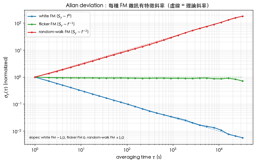
lab_19 (simulations/lab_19_allan.py) generates the fractional frequency $y(t)$ for the three FM noise types by FFT shaping, integrates it into the time error $x(t)=\int y\,dt$, and then estimates the overlapping Allan deviation: for each $\tau=m\tau_0$, take the mean square of the second difference $x_{k+2m}-2x_{k+m}+x_k$ and the square root. In the figure, solid lines are the simulated ADEV, dashed lines the theoretical slopes; the three slopes land precisely on $-1/2$, $0$, and $+1/2$:

Item	Value	Notes
Model	toy / illustrative (not transistor-level)	synthesizes $S_y\sim f^\alpha$ by FFT power-law shaping
white FM	$S_y\sim f^{0}$	ADEV slope $\tau^{-1/2}$ (blue)
flicker FM	$S_y\sim f^{-1}$	ADEV slope $\tau^{0}$, flicker floor (green)
random-walk FM	$S_y\sim f^{-2}$	ADEV slope $\tau^{+1/2}$ (red)
Estimator	overlapping ADEV	second-difference kernel $x_{k+2m}-2x_{k+m}+x_k$
Vertical axis	normalized $\sigma_y/\sigma_y(\tau_0)$	compares slopes only; absolute scale arbitrary

Core Python (full script: simulations/lab_19_allan.py, function overlapping_adev):

import numpy as np

def overlapping_adev(x, tau0, ms):
    """Compute the overlapping Allan deviation from time-error samples x (spacing tau0)."""
    x = np.asarray(x); N = len(x); out = []
    for m in ms:
        if N - 2 * m < 1:
            out.append(np.nan); continue
        d = x[2 * m:] - 2 * x[m:-m] + x[:-2 * m]      # second difference of the time error
        avar = np.sum(d ** 2) / (2 * (N - 2 * m) * (m * tau0) ** 2)
        out.append(np.sqrt(avar))
    return np.array(out)

The d line is the second difference $x_{k+2m}-2x_{k+m}+x_k$ of Step 2; dividing by $2(N-2m)(m\tau_0)^2$ corresponds to the discrete estimate of $\sigma_y^2=\langle\tfrac12(\bar y_{k+1}-\bar y_k)^2\rangle$ (with $\tau=m\tau_0$).

Interactive: generate your own time series and estimate ADEV yourself (statistics vs. analytic)

The lab_19 figure above tells you the three slopes a priori. In practice, though, you only ever have one finite-length measured time series, and ADEV is a statistic estimated from that series — not an analytic curve handed down from above. The widget below moves the full "generate → estimate" pipeline into the browser, complementing the AllanDeviationExplorer on the interactive_calculator page (which plots the pure analytic slope with no randomness at all):

• A seeded pseudo-random number generator (PRNG — meaning the same seed always reproduces the same series) generates a fractional-frequency series $y[k]$ of length $N=4096$, made of slider-controlled white FM + random-walk FM, plus an optional flicker FM approximated with a simple $-10$dB/decade filter cascade (an honest approximation — see the note below).
• The series is integrated into a time error $x[k]=\sum y[k]\tau_0$, and the same overlapping second-difference formula from Steps 2–3 is applied to estimate ADEV directly at $\tau=\tau_0,2\tau_0,4\tau_0,\dots$ (octaves, up to $N/4$), with $\pm\sigma/\sqrt{\text{pairs}}$ error bars overlaid.
• The dashed line is the analytic closed form for the same mixture of $h$ coefficients (Step 4 / the prefactor table, variances of independent processes add) — the blue points should scatter around it.
• Click "re-seed" to draw a new seed: the small-$\tau$ points barely move (thousands of independent pairs, statistically stable), while the large-$\tau$ points visibly jump around (only about 4 independent pairs remain at $\tau=N/4$). This is exactly the lesson of this section: the "floor" or "upturn" you see at the far right of an ADEV curve can look like a definite physical feature, but if it is only supported by a handful of independent samples, those last few points carry large statistical uncertainty of their own — the fix is a longer total record, not taking the shape of the rightmost points at face value.

Live ADEV from a synthetic time series (N=4096) — statistics vs. analytic

Generates one fractional-frequency series y[k] with a seeded PRNG, integrates it to a time error x[k], then estimates overlapping ADEV directly (second-difference of x) at each octave τ = m·τ₀. The dashed line is the analytic closed form for the same mixture (variances add).

white FM level h₀ = 10^x-19.0

random-walk FM level h₋₂ = 10^x-24.0

seed = 1234

largest τ pairs

2048

τ = 1024

smallest τ measured/theory

0.993

(white-FM-only closed form)

Estimator: overlapping ADEV σ_y²(mτ₀) = Σᵢ(x[i+2m]−2x[i+m]+x[i])² / (2·pairs·(mτ₀)²), the discrete second difference of the time error x = ∫y dt (identical formula to lab_19 / the analytic page above). Error bars use the rule-of-thumb ±σ/√pairs — a simplification (overlapping windows are correlated, so this understates the true uncertainty somewhat), but it correctly shows the qualitative point: the largest τ has few independent windows (N/τ ~ 4 at τ=N/4), so its ADEV point is noisy and jumps a lot between re-seeds, while small-τ points (thousands of pairs) are stable run to run. Flicker FM here is only an honest approximation: a cascade of 8 log-spaced one-pole (leaky-integrator) filters gives an effective PSD slope around −0.8 to −0.9 decade⁻¹ (not the exact −1 of true 1/f) over the covered band — good enough to see the τ⁰ floor bend into view, not a rigorous flicker generator. Verified in Node against a pure white-FM case (h₀=10⁻¹⁹, random-walk and flicker off): averaged over 200 reseeds the measured/theory ratio is 0.94–1.00 across all 11 octaves (worst at the largest τ, where pairs are scarcest — see below), and the fitted log–log slope of the seed-averaged curve is −0.508 (expected −1/2); a single seed (default seed 1234) already gives ratio 0.993 at the smallest τ.

Independent check of the estimator: switching the generator to pure white FM (random-walk and flicker off) with $h_0=10^{-19}$ and running the same algorithm in Node over 200 re-seeds, the measured/theory ratio (against the closed form $h_0/2\tau$) at every octave of $\tau$ falls in the range $0.94$–$1.00$ (worst at the largest $\tau$, where pairs are scarcest — exactly the effect described above); the log–log slope fitted to the 200-seed-averaged curve is $-0.508$ (theory: $\tau^{-1/2}$), and a single run with the default seed (1234) already gives a ratio of $0.993$ at the smallest $\tau$. The widget's "smallest τ measured/theory" readout is a live version of this same self-check.

Worked examples

The two problems below follow the strict format: problem → step-by-step substitution (with units) → result → dimension check → one-line Python verification. The first practices "reading slopes off the plot"; the second demonstrates estimating ADEV from $\mathcal{L}(f)$ (the most useful engineering conversion).

Example 1: reading the noise type from two ADEV points and extrapolating

Problem: an OCXO (oven-controlled crystal oscillator) measures $\sigma_y(1\,\text{s})=2\times10^{-12}$ and $\sigma_y(10\,\text{s})=6.3\times10^{-13}$. Which noise type dominates in this range? Extrapolate $\sigma_y(100\,\text{s})$.

Steps:

1. Compute the slope $\mu$ ($\sigma_y\propto\tau^\mu$):

$$\mu=\frac{\log_{10}\!\big(\sigma_y(10)/\sigma_y(1)\big)}{\log_{10}(10/1)}=\frac{\log_{10}(6.3\times10^{-13}/2\times10^{-12})}{\log_{10}10}=\frac{\log_{10}(0.315)}{1}\approx-0.5.$$

2. Consulting the Step-4 table: $\mu=-1/2$ ⇒ white FM dominates ($S_y\sim f^0$, equivalently $S_\phi\sim1/f^2$).
3. Extrapolate to $\tau=100\,\text{s}$ (still white FM, $\tau^{-1/2}$):

$$\sigma_y(100)=\sigma_y(1)\times(100)^{-1/2}=2\times10^{-12}\times\frac{1}{10}=2\times10^{-13}.$$

Result: white FM dominates; $\sigma_y(100\,\text{s})\approx2\times10^{-13}$.

Dimension check: $\sigma_y$ is dimensionless throughout (fractional frequency); the slope $\mu$ is a ratio of logs of two dimensionless quantities, hence dimensionless ✓.

import numpy as np
mu = np.log10(6.3e-13/2e-12)/np.log10(10)          # -> -0.50  => white FM
adev_100 = 2e-12*(100/1)**mu
print(round(mu,2), f"{adev_100:.2e}")              # -> -0.5  2.00e-13

Example 2: estimating ADEV from the white-noise $1/f^2$ region of $\mathcal{L}(f)$

Problem: a 5 GHz oscillator measures $\mathcal{L}(1\,\text{MHz})=-100\,\text{dBc/Hz}$ in the 1/f² region (the white-FM segment). Estimate how $\sigma_y(\tau)$ scales with $\tau$, and give the numerical value of $\sigma_y(1\,\text{ms})$. Uses the setup of canonical Example C ($f_0=5\,\text{GHz}$).

Steps:

1. dBc/Hz → linear $\mathcal{L}$: $\mathcal{L}(1\,\text{MHz})=10^{-100/10}=10^{-10}\,\text{rad}^2/\text{Hz}$ (single-sided).
2. $\mathcal{L}\to S_\phi$ (small-angle $\mathcal{L}\approx\tfrac12 S_\phi$, see spec Eq.16): $S_\phi(1\,\text{MHz})=2\mathcal{L}=2\times10^{-10}\,\text{rad}^2/\text{Hz}$.
3. Write the explicit $1/f^2$ form: in the white-FM segment $S_\phi(f)=\dfrac{h_{-2}}{f^2}$. Substituting $f=10^6$: $h_{-2}=S_\phi(10^6)\cdot(10^6)^2=2\times10^{-10}\times10^{12}=2\times10^{2}=200\,\text{rad}^2\,\text{Hz}$.
4. Convert to $S_y$: $S_y(f)=\dfrac{f^2}{f_0^2}S_\phi=\dfrac{f^2}{f_0^2}\cdot\dfrac{h_{-2}}{f^2}=\dfrac{h_{-2}}{f_0^2}\equiv h_0$ (white indeed — independent of $f$). $h_0=\dfrac{200}{(5\times10^9)^2}=\dfrac{200}{2.5\times10^{19}}=8.0\times10^{-18}\,\text{Hz}^{-1}$.
5. Closed form of ADEV for white FM (a standard result, obtained by integrating the Step-3 kernel with $S_y=h_0$):

$$\sigma_y^2(\tau)=\frac{h_0}{2\tau}\quad\Longrightarrow\quad\sigma_y(\tau)=\sqrt{\frac{h_0}{2\tau}}.$$

6. Substituting $\tau=10^{-3}\,\text{s}$: $\sigma_y^2=\dfrac{8.0\times10^{-18}}{2\times10^{-3}}=4.0\times10^{-15}$, $\sigma_y=6.3\times10^{-8}$.

Result: $S_y$ is white with $h_0=8.0\times10^{-18}\,\text{Hz}^{-1}$; $\sigma_y(\tau)=\sqrt{h_0/2\tau}\propto\tau^{-1/2}$ (consistent with white FM); $\sigma_y(1\,\text{ms})\approx6.3\times10^{-8}$.

Dimension check: $h_0$ has units $\text{Hz}^{-1}=\text{s}$; $h_0/\tau$ is dimensionless; the square root remains dimensionless → $\sigma_y$ dimensionless ✓. The slope $\sigma_y\propto\tau^{-1/2}$ matches the white-FM row of the table ✓.

Feel for the numbers: $6.3\times10^{-8}$ looks large at 1 ms, but a free-running 5 GHz oscillator does drift away a lot of phase within 1 ms (which is exactly why a PLL/CDR is used to pin the long-term frequency; see serdes_clocking_connection). Stretch $\tau$ to 1 s and $\sigma_y$ drops by another factor $\sqrt{1000}\approx31.6$ to $\sim2\times10^{-9}$.

import numpy as np
f0, L_dbc, foff = 5e9, -100.0, 1e6
S_phi = 2*10**(L_dbc/10)                 # rad^2/Hz at foff (small-angle L≈½S_φ)
h_2   = S_phi*foff**2                     # S_phi = h_2/f^2  => h_2
h0    = h_2/f0**2                         # S_y = h0 (white FM)
adev  = lambda tau: np.sqrt(h0/(2*tau))
print(f"{h0:.1e}", f"{adev(1e-3):.1e}")  # -> 8.0e-18  6.3e-08

(The white-FM closed form $\sigma_y^2=h_0/2\tau$ is a standard frequency-metrology result — the next section derives it fully in-house using $I_2=\pi/4$, and lab_19 has been extended to verify the absolute level as well, not just the slope.)

The complete prefactor table: the flicker-FM floor constant $\sigma_y^2=2\ln 2\cdot h_{-1}$

The Step-4 slope table only answers "$\sigma_y\propto\tau^\mu$" — it says nothing about the absolute level. What engineering actually needs is: given the power-law coefficients of $S_y$, the exact numerical value of each segment of the ADEV curve — above all, how high the flicker-FM floor sits, the level that "no amount of averaging gets you below". This section evaluates the Step-3 integral for each of the five power laws one by one: the centerpiece is the flicker-FM floor constant, which turns out to be a beautiful $\ln 2$; white FM and RW FM fall to the same trick along the way; and the two PM types will show us "why a high-frequency cutoff $f_h$ is unavoidable".

Notation: the power-law coefficients $h_\alpha$ (standard IEEE 1139 notation)

The frequency-metrology standards write $S_y$ as a power-law superposition:

$$S_y(f)=\sum_{\alpha=-2}^{+2}h_\alpha f^{\alpha}.$$

$S_y$ has units $1/\text{Hz}$, so $h_\alpha$ has units $\text{Hz}^{-(\alpha+1)}$: $h_{+2}$ is $\text{Hz}^{-3}$, $h_{+1}$ is $\text{Hz}^{-2}$, $h_0$ is $\text{Hz}^{-1}=\text{s}$, $h_{-1}$ is dimensionless, $h_{-2}$ is $\text{Hz}$.

Notation warning: the $h_\alpha$ always attach to $S_y$ (the standard IEEE 1139 usage). In Example 2 above we casually wrote the $1/f^2$ coefficient of $S_\phi$ as $h_{-2}$ — that is the $S_\phi$-side coefficient, not the same object as the RW-FM $h_{-2}$ here (which lives on the $S_y$ side, with units Hz). From this section on, $S_\phi$-side coefficients carry a superscript $\phi$: the white-FM segment is written $S_\phi=h^{\phi}_{-2}/f^2$ (with $h^{\phi}_{-2}$ in $\text{rad}^2\cdot\text{Hz}$).

The general formula: one substitution covers all five rows

Substitute $S_y=h_\alpha f^\alpha$ into the Step-3 integral and change variables $u=\pi f\tau$ (dimensionless; $f=u/(\pi\tau)$, $df=du/(\pi\tau)$, $f^\alpha=u^\alpha/(\pi\tau)^\alpha$):

$$\sigma_y^2(\tau)=2\int_0^{\infty}h_\alpha f^{\alpha}\,\frac{\sin^4(\pi f\tau)}{(\pi f\tau)^2}\,df =\frac{2\,h_\alpha}{(\pi\tau)^{\alpha+1}}\,I_{2-\alpha}, \qquad I_k\equiv\int_0^{\infty}\frac{\sin^4 u}{u^{k}}\,du.$$

• Step by step: the integrand $=h_\alpha\dfrac{u^\alpha}{(\pi\tau)^\alpha}\cdot\dfrac{\sin^4u}{u^2}\cdot\dfrac{du}{\pi\tau}=h_\alpha\,(\pi\tau)^{-(\alpha+1)}\,\dfrac{\sin^4u}{u^{2-\alpha}}\,du$; pull out the constants and the result follows.
• The slope table comes out for free: $\sigma_y^2\propto\tau^{-(\alpha+1)}$ — $\alpha=0\Rightarrow\tau^{-1}$ (white FM), $\alpha=-1\Rightarrow\tau^{0}$ (floor), $\alpha=-2\Rightarrow\tau^{+1}$ (RW FM), consistent with the Step-4 table ✓. All that remains is to evaluate the pure numbers $I_k$.
• Convergence (important): as $u\to0$ the integrand $\sim u^{4-k}$ ($k=2-\alpha\le4$, integrable for all $\alpha\ge-2$ ✓); as $u\to\infty$ it goes $\sim u^{-k}$, requiring $k>1$, i.e. $\alpha<1$. For $\alpha=+1,+2$ (the two PM types) the integral diverges at the high-frequency end — physically: the ADEV of PM noise depends on how high a frequency the measurement system can see, so a high-frequency cutoff $f_h$ (Hz) must be introduced, truncating at $u_h=\pi f_h\tau$. This is the deeper reason why the two PM rows of the Step-4 table cannot do without $f_h$.
• Unit check: $h_\alpha$ is $\text{Hz}^{-(\alpha+1)}$, $(\pi\tau)^{-(\alpha+1)}$ is $\text{Hz}^{+(\alpha+1)}$, $I_k$ is a pure number ⇒ $\sigma_y^2$ dimensionless ✓.

Flicker FM ($\alpha=-1$): proving $I_3=\ln 2$

For $\alpha=-1$ we get $(\pi\tau)^{\alpha+1}=(\pi\tau)^{0}=1$ — $\tau$ disappears entirely at the very first step; the "$\tau$-independence" of the floor is established right here, before evaluating any integral:

$$\sigma_y^2(\tau)=2\,h_{-1}\,I_3=2\,h_{-1}\int_0^{\infty}\frac{\sin^4u}{u^3}\,du.$$

All that is left is the pure number $I_3$. Four sub-steps below, no jumps.

Step (i): power-reduce $\sin^4$ into harmonics. Square $\sin^2u=\tfrac12(1-\cos2u)$, then use $\cos^2 2u=\tfrac12(1+\cos4u)$:

$$\sin^4u=\frac{(1-\cos2u)^2}{4}=\frac{1-2\cos2u+\cos^2 2u}{4}=\frac{3-4\cos2u+\cos4u}{8}=\frac{4(1-\cos2u)-(1-\cos4u)}{8}.$$

Check the last equality: $4-4\cos2u-1+\cos4u=3-4\cos2u+\cos4u$ ✓. Small-$u$ check: $1-\cos(au)=\tfrac{a^2u^2}{2}-\tfrac{a^4u^4}{24}+\dots$; the $u^2$ coefficient $4\cdot\tfrac{4}{2}-\tfrac{16}{2}=8-8=0$ cancels, and the $u^4$ term $-4\cdot\tfrac{16}{24}+\tfrac{256}{24}=8$ gives the combination $\approx8u^4=8\sin^4u$ ✓ ($\sin^4u\approx u^4$).

Step (ii): why we must group into "$(1-\cos)$ combinations" and may not split. If you integrate $3-4\cos2u+\cos4u$ against $u^{-3}$ term by term, each piece $\dfrac{1-\cos(au)}{u^3}\approx\dfrac{a^2}{2u}$ diverges logarithmically as $u\to0$; only in the combination does the $1/u$ coefficient $4\cdot\tfrac{2^2}{2}-\tfrac{4^2}{2}=0$ cancel exactly, making the whole thing integrable (low end $\sin^4u/u^3\sim u\to0$, high end $\le1/u^3$ ✓). So below we treat it as a whole and never split — this "individually divergent, finite in combination" structure is exactly the usual temperament of $1/f$ noise (compare Step 5: the standard variance diverges while the differenced combination converges).

Step (iii): integrate by parts twice, lowering $u^{-3}$ to $u^{-1}$. Write $g(u)\equiv8\sin^4u=3-4\cos2u+\cos4u$, so $I_3=\tfrac18\int_0^\infty g(u)\,u^{-3}du$.

First integration by parts ($u^{-3}du=d(-\tfrac{1}{2u^2})$):

$$\int_0^{\infty}\frac{g(u)}{u^3}\,du=\Big[-\frac{g(u)}{2u^2}\Big]_0^{\infty}+\frac12\int_0^{\infty}\frac{g'(u)}{u^2}\,du, \qquad g'(u)=8\sin2u-4\sin4u.$$

Boundary terms: as $u\to\infty$, $\lvert g\rvert\le8$ ⇒ $g/u^2\to0$; as $u\to0$, $g\approx8u^4$ ⇒ $g/(2u^2)\approx4u^2\to0$ ✓ both ends vanish.

Second integration by parts ($u^{-2}du=d(-u^{-1})$):

$$\int_0^{\infty}\frac{g'(u)}{u^2}\,du=\Big[-\frac{g'(u)}{u}\Big]_0^{\infty}+\int_0^{\infty}\frac{g''(u)}{u}\,du, \qquad g''(u)=16\cos2u-16\cos4u.$$

Boundary terms: at the $\infty$ end $g'$ is bounded ⇒ $g'/u\to0$; at the $0$ end $g'=8\sin2u-4\sin4u=(16u-16u)+O(u^3)=32u^3+O(u^5)$ ⇒ $g'/u\approx32u^2\to0$ ✓. Combining:

$$I_3=\frac18\cdot\frac12\int_0^{\infty}\frac{16(\cos2u-\cos4u)}{u}\,du=\int_0^{\infty}\frac{\cos2u-\cos4u}{u}\,du.$$

Step (iv): a Frullani-type cosine integral → $\ln2$. Each term alone diverges as $u\to0$ ($\int du/u$), but the combination is integrable ($\cos2u-\cos4u=6u^2+O(u^4)$, integrand $\sim6u\to0$). Take a lower limit $\varepsilon>0$ and substitute $v=2u$ and $v=4u$ in the two terms respectively:

$$\int_{\varepsilon}^{\infty}\frac{\cos2u-\cos4u}{u}\,du=\int_{2\varepsilon}^{\infty}\frac{\cos v}{v}\,dv-\int_{4\varepsilon}^{\infty}\frac{\cos v}{v}\,dv=\int_{2\varepsilon}^{4\varepsilon}\frac{\cos v}{v}\,dv.$$

(At the $\infty$ end each integral converges conditionally — Dirichlet's test — and the identical tails cancel on subtraction, leaving only the sliver $[2\varepsilon,4\varepsilon]$.) On that sliver $\lvert\cos v-1\rvert\le v^2/2$:

$$\int_{2\varepsilon}^{4\varepsilon}\frac{\cos v}{v}\,dv=\int_{2\varepsilon}^{4\varepsilon}\frac{dv}{v}+O(\varepsilon^2)=\ln\frac{4\varepsilon}{2\varepsilon}+O(\varepsilon^2)\ \xrightarrow{\ \varepsilon\to0\ }\ \ln2.$$

Therefore:

$$\boxed{\ I_3=\int_0^{\infty}\frac{\sin^4u}{u^3}\,du=\ln2 \quad\Longrightarrow\quad \sigma_y^2(\tau)=2\ln2\cdot h_{-1}\ (\text{independent of }\tau),\quad \sigma_{y,\text{floor}}=\sqrt{2\ln2\cdot h_{-1}}\approx1.1774\,\sqrt{h_{-1}}\ }$$

Physical intuition: $\ln2=\ln\frac{4}{2}$ is the log of the frequency ratio of the two harmonics $2u$ and $4u$ produced by the power reduction. A $1/f$ process contributes equal power per octave; the ADEV band-pass kernel, on a log-frequency axis, is a window of fixed shape that merely slides with $\tau$ (weighted by $S_y\sim1/f$, the contribution density per decade is $\propto\sin^4u/u^2$, peaking at $\tan u=2u$, i.e. $u\approx1.17$, $f\approx0.37/\tau$) — the window slides without changing shape, so the "number of octaves" it sees does not depend on $\tau$, and the integral is a constant. That is the frequency-domain picture of why the flicker floor is "$\tau$-independent".

Numerical verification (scipy.integrate.quad up to $200\pi$ plus the analytic $\langle\sin^4\rangle=3/8$ tail correction; printed by lab_19):

import numpy as np
from scipy.integrate import quad
U = 200*np.pi
I3, _ = quad(lambda u: np.sin(u)**4/u**3, 0, U, limit=4000)
I3 += (3/8)/(2*U**2)                  # tail ∫_U^∞ (3/8)/u^3 du
print(f"{I3:.4f} {np.log(2):.4f}")    # -> 0.6931 0.6931

Factor-2/4 bookkeeping (the origin of every 2 and 4 in this section, settled once and for all):

• The leading 2 in $\sigma_y^2=2\ln2\cdot h_{-1}$: from the Step-3 kernel $\lvert H\rvert^2=2\sin^4u/u^2$ (the definition's $\tfrac12$ × the adjacent-difference $4\sin^2$) — this is ADEV mathematics, and has nothing to do with the phase-noise SSB $/2$-vs-$/4$ bookkeeping.
• The 2 and 4 in $\cos2u$ and $\cos4u$: the second and fourth harmonics from power-reducing $\sin^4$; $\ln2=\ln(4/2)$ is precisely their frequency ratio.
• The 2 in the white-FM denominator $h_0/(2\tau)$: $2\cdot\frac{I_2}{\pi}=2\cdot\frac{\pi/4}{\pi}=\frac12$ — again ADEV mathematics, not SSB bookkeeping.
• The $4\pi^2$ in the denominator of $h^{\phi}_{-2}$ in Example 3 below: from $(2\pi f)^2$, purely the rad ↔ Hz conversion.
• The 4 in the denominator of $\tau_{knee}$ in Example 3: $=2\times2$ (the 2 of $h_0/\mathbf{2}\tau$ × the 2 of $\mathbf{2}\ln2$).
• The genuine SSB $/2$-vs-$/4$ convention appears only when "converting $S_\phi$ into a dBc/Hz report" (flagged in Example 3, Step 1).

The same trick takes down white FM and RW FM (and the $f_h$ of the two PM rows)

White FM ($\alpha=0$): $\sigma_y^2=\dfrac{2h_0}{\pi\tau}I_2$. $I_2$ needs only one integration by parts (the boundary terms again vanish at both ends: $\sin^4u/u\sim u^3\to0$ and $\le1/u\to0$):

$$I_2=\int_0^{\infty}\frac{\sin^4u}{u^2}\,du=\Big[-\frac{\sin^4u}{u}\Big]_0^{\infty}+\int_0^{\infty}\frac{4\sin^3u\cos u}{u}\,du=\int_0^{\infty}\frac{\sin2u-\tfrac12\sin4u}{u}\,du=\frac{\pi}{2}-\frac12\cdot\frac{\pi}{2}=\frac{\pi}{4}.$$

(In the middle we used $4\sin^3u\cos u=2\sin2u\sin^2u=\sin2u(1-\cos2u)=\sin2u-\tfrac12\sin4u$, plus the Dirichlet integral $\int_0^\infty\frac{\sin(au)}{u}du=\frac{\pi}{2}$, $a>0$.) Substituting back:

$$\sigma_y^2(\tau)=\frac{2h_0}{\pi\tau}\cdot\frac{\pi}{4}=\frac{h_0}{2\tau}.$$

The "standard result" quoted in Example 2 is thereby derived in-house ✓.

RW FM ($\alpha=-2$): $\sigma_y^2=2h_{-2}(\pi\tau)\,I_4$, where $I_4=\int_0^\infty\sin^4u/u^4\,du=\dfrac{\pi}{3}$ (same family: three integrations by parts reduce it to the Dirichlet family; it is also in the standard integral tables, and lab_19 verifies 1.0472 $=\pi/3$ by quad). Substituting back:

$$\sigma_y^2(\tau)=2\pi\tau\,h_{-2}\cdot\frac{\pi}{3}=\frac{2\pi^2}{3}\,h_{-2}\,\tau.$$

The two PM rows ($\alpha=+1,+2$): $I_1,I_0$ diverge as $u\to\infty$; truncate at $u_h=\pi f_h\tau$. For white PM use $\int_0^{u_h}\sin^4u\,du=\tfrac38u_h-\tfrac14\sin2u_h+\tfrac1{32}\sin4u_h\approx\tfrac38u_h$ ($u_h\gg1$, $\langle\sin^4\rangle=3/8$):

$$\sigma_y^2\approx\frac{2h_{+2}}{(\pi\tau)^3}\cdot\frac38\,\pi f_h\tau=\frac{3\,f_h\,h_{+2}}{4\pi^2\tau^2},$$

which is exactly the standard white-PM prefactor (condition $2\pi f_h\tau\gg1$) ✓. Flicker PM works the same way: the logarithmic divergence of $I_1$ produces the $\langle\sin^4\rangle\cdot\ln$ term with coefficient $\tfrac{3}{4\pi^2\tau^2}$; the additive constant $1.038$ requires more careful oscillatory bookkeeping, so this page quotes the standard value directly (external literature).

The complete prefactor table for the five power laws

Noise type	$S_y(f)$	Units of $h_\alpha$	$\sigma_y^2(\tau)$	Condition	Source
white PM	$h_{+2}f^{2}$	$\text{Hz}^{-3}$	$\dfrac{3\,f_h\,h_{+2}}{4\pi^2\tau^2}$	$2\pi f_h\tau\gg1$	standard table; prefactor derived here via $\langle\sin^4\rangle=\tfrac38$
flicker PM	$h_{+1}f$	$\text{Hz}^{-2}$	$\dfrac{\big[1.038+3\ln(2\pi f_h\tau)\big]h_{+1}}{4\pi^2\tau^2}$	$2\pi f_h\tau\gg1$	standard table; $\ln$ coefficient derived here, constant 1.038 quoted
white FM	$h_0$	$\text{Hz}^{-1}=\text{s}$	$\dfrac{h_0}{2\tau}$	—	derived in-house ($I_2=\pi/4$)
flicker FM	$h_{-1}/f$	dimensionless	$2\ln2\cdot h_{-1}$ ($\approx1.386\,h_{-1}$, floor)	—	derived in-house ($I_3=\ln2$)
random-walk FM	$h_{-2}/f^{2}$	$\text{Hz}$	$\dfrac{2\pi^2}{3}\,h_{-2}\,\tau$	—	derived in-house ($I_4=\pi/3$)

$f_h$ = high-frequency cutoff of the measurement system (Hz). The whole table agrees entry by entry with the standard tables of IEEE Std 1139-2008 and NIST SP 1065 (W. J. Riley, Handbook of Frequency Stability Analysis, 2008) (external literature, not among this site's 5 source PDFs); the flicker-FM, white-FM, and RW-FM rows and the white-PM prefactor have been derived on this page. Per-row unit self-check: every combination of the form $h_\alpha\,\text{Hz}^{(\alpha+1)}$ is dimensionless ✓ (e.g. RW FM: $\text{Hz}\times\text{s}$ ✓; flicker PM: $\text{Hz}^{-2}/\text{s}^2$ ✓).

Example 3: computing the flicker floor from the canonical $1/f^3$ corner (with units)

Problem: the canonical oscillator ($f_0=5$ GHz, $q_{max}=1$ pC, $\Gamma_{rms}=0.5$, $S_i=10^{-24}\ \text{A}^2/\text{Hz}$), with waveform symmetrized so that $c_0=0.04$; Example F of flicker_noise_upconversion gives the $1/f^3$ corner $f_c=3.2$ kHz. Find the flicker-FM floor $\sigma_{y,\text{floor}}$ and the $\tau_{knee}$ where the white-FM segment crosses the floor.

Step 1 (the physical $S_\phi$ of the white-FM segment): the time-domain-clean derivation (see the factor-of-2 note in white_noise_to_phase_noise) gives the single-sided

$$S_\phi(f)=\frac{\Gamma_{rms}^2}{q_{max}^2}\cdot\frac{S_i}{(2\pi f)^2}=\frac{h^{\phi}_{-2}}{f^2}, \qquad h^{\phi}_{-2}=\frac{\Gamma_{rms}^2\,S_i}{4\pi^2\,q_{max}^2}=\frac{0.25\times10^{-24}}{4\pi^2\times10^{-24}}=6.33\times10^{-3}\ \text{rad}^2\cdot\text{Hz}.$$

• Unit check: $\text{A}^2/\text{Hz}\div\text{C}^2=(\text{C/s})^2/(\text{Hz}\cdot\text{C}^2)=\text{Hz}^2/\text{Hz}=\text{Hz}$, times the dimensionless $\Gamma_{rms}^2$ gives $\text{rad}^2\cdot\text{Hz}$ ✓ (the $4\pi^2$ in the denominator comes from $(2\pi f)^2$ — a rad↔Hz conversion, not a noise-bookkeeping convention).
• Convention flag (every single time): this is the physical single-sided $S_\phi$. When converted into a dBc/Hz report: the time-domain $/2$ convention ($\mathcal{L}=S_\phi/2$) gives $\mathcal{L}(1\,\text{MHz})=-145.0$ dBc/Hz, while the SSB $/4$ accounting of [P1] Eq.(21) gives $-148.0$ dBc/Hz (a 3 dB difference; canonical Example B). ADEV consumes only the physical $S_\phi$, so this example corresponds to the $-145$ reading; if you mistakenly invert $-148$ as $S_\phi/2$, your $h^{\phi}_{-2}$ comes out 2× too small and the floor $\sqrt2$ too low ($-1.5$ dB).

Step 2 (flicker segment → $h_{-1}$): below the corner, $S_\phi$ steepens to $1/f^3$, continuous with the white-FM segment at $f_c$: $S_\phi=\dfrac{h^{\phi}_{-2}\,f_c}{f^3}$ ($f<f_c$). Converting to $S_y$ (the Step-1 adapter):

$$S_y(f)=\frac{f^2}{f_0^2}\,S_\phi=\frac{h^{\phi}_{-2}\,f_c}{f_0^2}\cdot\frac1f\equiv\frac{h_{-1}}{f}, \qquad h_{-1}=\frac{h^{\phi}_{-2}\,f_c}{f_0^2}=\frac{6.33\times10^{-3}\times3.2\times10^{3}}{(5\times10^{9})^2}=8.11\times10^{-19}.$$

• Unit check: $\text{rad}^2\cdot\text{Hz}\times\text{Hz}\div\text{Hz}^2=$ dimensionless ✓ ($h_{-1}$ should be dimensionless).
• Worth noting: $h_{-1}=h_0\,f_c$, where $h_0=h^{\phi}_{-2}/f_0^2=2.53\times10^{-22}\ \text{Hz}^{-1}$ is the white-FM level — the flicker coefficient is just "white-FM level × corner frequency".

Step 3 (the floor):

$$\sigma_{y,\text{floor}}=\sqrt{2\ln2\cdot h_{-1}}=\sqrt{1.3863\times8.11\times10^{-19}}=\sqrt{1.124\times10^{-18}}=1.06\times10^{-9}.$$

Result: the floor is $\approx1.06\times10^{-9}$, about 1.1 ppb — in frequency terms: $\sigma_y f_0=1.06\times10^{-9}\times5\times10^{9}=5.3$ Hz. No matter how long you average, the two-sample frequency instability of this free-running oscillator is stuck at about 5.3 Hz — that is the engineering meaning of the flicker floor.

Step 4 (the knee: where the white-FM segment hits the floor): set $h_0/(2\tau)=2\ln2\cdot h_{-1}$ and use $h_{-1}=h_0f_c$:

$$\tau_{knee}=\frac{h_0}{4\ln2\cdot h_{-1}}=\frac{1}{4\ln2\cdot f_c}=\frac{0.3607}{f_c}=\frac{0.3607}{3200\ \text{Hz}}=113\ \mu\text{s}.$$

(The 4 in the denominator $=2\times2$: the 2 of $h_0/\mathbf{2}\tau$ × the 2 of $\mathbf{2}\ln2$, both ADEV mathematics.) For $\tau$ shorter than 113 μs white FM dominates (the $\tau^{-1/2}$ descent); beyond it you sit on the floor. Rule of thumb: $\tau_{knee}\approx0.36/f_c$.

Contrast (asymmetric waveform): Example E's $c_0=0.4$ gives $f_c=320$ kHz ⇒ $h_{-1}=8.11\times10^{-17}$, floor $=1.06\times10^{-8}$. The corner is 100× higher, the floor only 10× higher (the $\sqrt{\ }$), and the knee shrinks to 1.13 μs. Because $f_c\propto c_0^2$ ([P1] Eq.(24)) while the floor $\propto\sqrt{h_{-1}}\propto\sqrt{f_c}$, we get floor $\propto c_0$: waveform symmetrization does not just suppress close-in phase noise — it pulls the long-term-stability floor down linearly in $c_0$.

Dimension check (throughout): $h_{-1}$ dimensionless → $2\ln2\,h_{-1}$ dimensionless → the square root still dimensionless (fractional frequency) ✓; $\tau_{knee}=h_0/(4\ln2\,h_{-1})=\text{s}/\text{dimensionless}=\text{s}$ ✓.

import numpy as np
g, Si, qmax, f0, fc = 0.5, 1e-24, 1e-12, 5e9, 3.2e3
h_phi = g**2*Si/(qmax**2*4*np.pi**2)          # S_phi white-FM coefficient (rad^2·Hz)
h_m1  = h_phi*fc/f0**2                        # S_y = h_m1/f (dimensionless)
floor = np.sqrt(2*np.log(2)*h_m1)
print(f"{h_phi:.2e} {h_m1:.2e} {floor:.2e}")  # -> 6.33e-03 8.11e-19 1.06e-09
h0 = h_phi/f0**2
print(f"{h0:.2e} {1/(4*np.log(2)*fc)*1e6:.0f}")  # -> 2.53e-22 113

Simulation verification: the absolute floor level (lab_19 extension)

lab_19 (simulations/lab_19_allan.py) has been extended to verify absolute values, not just slopes, doing three things:

1. The integral family: scipy.integrate.quad computes $I_2,I_3,I_4$ directly (up to $200\pi$ plus the analytic $\langle\sin^4\rangle=3/8$ tail), printing 0.7854, 0.6931, 1.0472, matching $\pi/4$, $\ln2$, $\pi/3$ ✓.
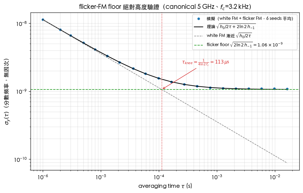
2. The floor of pure flicker FM: FFT shaping synthesizes $y(t)$ with an exactly known absolute PSD — unit-variance white noise has one-sided PSD $2/f_s$, so shape with $\lvert H\rvert^2=S_{target}/(2/f_s)$ (function synth_y_from_psd; unlike power_law_y, which normalizes only the slope) — with $h_{-1}=8.11\times10^{-19}$, 8 seeds, overlapping ADEV over $\tau=10\dots2000$ s, yielding measured/theory $=1.004$ (theory $\sqrt{2\ln2\,h_{-1}}=1.06\times10^{-9}$).
3. The full white＋flicker curve: superposing $S_y=h_0+h_{-1}/f$ (both canonical coefficients), $f_s=1$ MHz, $2^{22}$ points, 6 seeds; the entire curve (knee included) deviates from $\sqrt{h_0/2\tau+2\ln2\,h_{-1}}$ by at most 2.3%.

Item	Value	Notes
Model	toy / illustrative (not transistor-level)	FFT shaping, absolute one-sided PSD exactly known
$h_0$	$2.53\times10^{-22}\ \text{Hz}^{-1}$	canonical white-FM level (Example 3, Step 2)
$h_{-1}$	$8.11\times10^{-19}$ (dimensionless)	canonical flicker coefficient ($f_c=3.2$ kHz)
Theory floor	$\sqrt{2\ln2\,h_{-1}}=1.06\times10^{-9}$	green dashed line
Measured/theory (floor)	$1.004$	pure flicker, average of 8 seeds
Max full-curve deviation	$2.3\%$	includes FFT low-frequency truncation bias at large $\tau$
$\tau_{knee}$	$113\ \mu$s (red dotted line)	$=1/(4\ln2\,f_c)$

How to read it: the simulated points (blue) descend along the white-FM asymptote $\sqrt{h_0/2\tau}$ with slope $-1/2$ at small $\tau$, turn at $\tau_{knee}=113\ \mu$s, then sit on the $1.06\times10^{-9}$ floor — the level agrees with theory to 0.4% (floor band). Two honest caveats: (a) the lowest frequency of the synthesized noise is truncated by the record length at $f_s/N$, so at the largest $\tau$ some flicker power is missing and the curve deviates slightly (included in the 2.3%); (b) this is a toy synthesis validating the "integral mathematics" — the floor level of a real oscillator is set by its real $f_c$ and $h^{\phi}_{-2}$.

Applicability and failure conditions

Condition	When it holds	What happens when it fails
Noise expressible as a power-law superposition	slope table reads off the type directly	with spurs (discrete spectral lines), ADEV shows $\tau$-periodic bumps and needs separate interpretation
Distinguishing white PM vs flicker PM	ADEV cannot (both $\tau^{-1}$)	switch to MDEV (modified Allan) to separate them
Data long enough, $\tau\ll$ total record length	estimate is reliable	as $\tau$ approaches the record length, few samples remain and confidence intervals blow up
Processes no lower-frequency than RW FM	ADEV converges	for processes below RW ($S_y\sim f^{-3}$ and steeper) ADEV also diverges; use the Hadamard variance
Measurement system itself clean enough	you measure the DUT	otherwise the left end (small $\tau$) is buried under the instrument's white PM
Floor formula $\sigma_y^2=2\ln2\,h_{-1}$: $S_y\sim1/f$ must cover the band the kernel sees ($f\approx0.37/\tau$, roughly ±1.5 decades)	floor is flat and its level accurate	with $\tau$ too close to $\tau_{knee}$ the white-FM contribution is not negligible (use the full form $h_0/2\tau+2\ln2\,h_{-1}$); at very large $\tau$ RW FM / drift overrides the floor
PM-row prefactors require $2\pi f_h\tau\gg1$	white/flicker PM prefactors hold	for $\tau$ so small that $2\pi f_h\tau\sim1$ the prefactors lose accuracy ($f_h$ = measurement high-frequency cutoff)

Which papers / formulas this maps to

• This page's ADEV definition, $\sigma_y^2=2\int S_y\sin^4(\pi f\tau)/(\pi f\tau)^2 df$, $S_y=(f^2/f_0^2)S_\phi$, and the slope table are all adopted verbatim from spec §11.2 "Allan variance / ADEV".
• External literature (not among the 5 downloaded source PDFs; supplied from standard references):
  • [E1] D. W. Allan, "Statistics of Atomic Frequency Standards," Proc. IEEE, vol. 54, no. 2, pp. 221–230, Feb. 1966. (the original ADEV proposal)
  • IEEE Std 1139 ("IEEE Standard Definitions of Physical Quantities for Fundamental Frequency and Time Metrology—Random Instabilities") and NIST Special Publication 1065 (W. Riley, "Handbook of Frequency Stability Analysis," 2008) — the standard references for the power-law slope table and the overlapping-ADEV estimator.
  • The above are IEEE Std 1139-2008 (prior edition 1139-1999) and NIST SP 1065 (W. J. Riley, Handbook of Frequency Stability Analysis, 2008); volume/issue and edition details have been verified.
• Connection to this site's frequency-domain results: $S_\phi\sim1/f^2$ ([P1] Eq.(21) of white_noise_to_phase_noise) ↔ white FM ↔ ADEV $\tau^{-1/2}$; $1/f^3$ ([P1] Eq.(23) of flicker_noise_upconversion) ↔ flicker FM ↔ ADEV $\tau^0$ floor.
• The complete prefactor table: the whole table agrees with IEEE Std 1139-2008 and NIST SP 1065 (external literature, not among this site's 5 source PDFs); of it, the flicker-FM $2\ln2$ ($I_3=\ln2$), the white-FM $h_0/2\tau$ ($I_2=\pi/4$), the RW-FM $\tfrac{2\pi^2}{3}h_{-2}\tau$ ($I_4=\pi/3$), and the white-PM prefactor are derived on this page, using nothing beyond the Step-3 integral; the flicker-PM additive constant 1.038 is quoted from the standard. The corner $f_c=3.2$ kHz of Example 3 comes from [P1] Eq.(24) (Example F of flicker_noise_upconversion).

Key takeaways

• ADEV $\sigma_y(\tau)$ is the time-domain counterpart of phase noise: from the same $S_\phi(f)$, first convert $S_y=(f^2/f_0^2)S_\phi$, then substitute into $\sigma_y^2(\tau)=2\int_0^\infty S_y\,\sin^4(\pi f\tau)/(\pi f\tau)^2\,df$.
• The essence of the definition $\sigma_y^2(\tau)=\langle\tfrac12(\bar y_{k+1}-\bar y_k)^2\rangle$ is the adjacent difference (a first difference, i.e. a high-pass) blocking slow drift and the unknown grand mean.
• Five power-law slopes: white/flicker PM $\tau^{-1}$, white FM $\tau^{-1/2}$, flicker FM $\tau^{0}$ (floor), RW FM $\tau^{+1/2}$; the ADEV plot is a bathtub — drop, bottom out, climb — with the most stable point $\tau_{\text{opt}}$ at the bottom.
• Signature link: $1/f^2$ phase noise ↔ white FM ↔ ADEV slope $-1/2$.
• Why ADEV: the ordinary frequency variance does not converge for flicker/RW (it diverges with measurement duration); ADEV's differencing kernel goes like $f^2$ as $f\to0$, taming the low-frequency divergence and yielding a repeatable stability metric.
• Example 2 shows how $\mathcal{L}(1\text{MHz})=-100$ dBc/Hz (5 GHz) yields a white $S_y$ and $\sigma_y(1\text{ms})\approx6.3\times10^{-8}$.
• Prefactors, not just slopes: the substitution $u=\pi f\tau$ gives $\sigma_y^2=2h_\alpha(\pi\tau)^{-(\alpha+1)}I_{2-\alpha}$; $I_2=\pi/4$, $I_3=\ln2$, $I_4=\pi/3$ ⇒ white FM $h_0/2\tau$, flicker floor $2\ln2\,h_{-1}$ ($\tau$-independent), RW FM $\tfrac{2\pi^2}{3}h_{-2}\tau$; the two PM rows must carry $f_h$ because $I_1,I_0$ diverge at high frequency.
• Where the $\ln2$ comes from: power-reduce $\sin^4$ into the $2u,4u$ harmonics, integrate by parts twice, then the Frullani-type $\int(\cos2u-\cos4u)/u\,du=\ln(4/2)$; quad verifies 0.6931 ✓.
• Canonical numbers (Example 3): $f_c=3.2$ kHz ⇒ $h_{-1}=8.11\times10^{-19}$, floor $=1.06\times10^{-9}$ ($\approx5.3$ Hz @ 5 GHz), $\tau_{knee}=1/(4\ln2 f_c)=113\ \mu$s ($\approx0.36/f_c$); floor $\propto c_0$ — symmetrization directly lowers the long-term stability floor. lab_19 measures measured/theory $=1.004$ on synthesized noise with exactly known absolute PSD.

Further reading

• The same thing in the frequency domain: psd_phase_noise_jitter
• Where $1/f^2$ comes from (the frequency-domain origin of white FM): white_noise_to_phase_noise
• $1/f^3$ ↔ flicker FM floor: flicker_noise_upconversion
• Why phase locking pins the long-term frequency: serdes_clocking_connection
• Stochastic processes and PSD fundamentals: stochastic_noise_basics