β: This English translation is in beta — the Traditional-Chinese original is the authoritative version.

Rigorous Derivation of the Jitter Kernels: TIE, N-period, cycle-to-cycle

Prerequisites: psd_phase_noise_jitter · stochastic_noise_basics · dsp_view_of_phase_noise ｜ Next: allan_variance · serdes_clocking_connection

psd_phase_noise_jitter already gave the "operational versions" of the three jitter weighting kernels; this page derives them rigorously from first principles, and answers the question that has been left hanging: what exactly is the prefactor? Which 2 belongs to which convention? The answer is calibrated with three independent rulers: (1) the step-by-step derivation, (2) exact agreement with the verified $\sigma_{\Delta\phi}=\kappa\sqrt{\Delta t}$ of [P2], (3) Monte-Carlo time-domain measurement (simulations/lab_24_jitter_kernels.py) — all three agree to ~0.1%.

This page supersedes the earlier external-convention TODO: this site previously marked the prefactor of the period-jitter kernel in worked_examples Example C3 as "external literature, to be confirmed". This page has now derived it from first principles and verified it by Monte Carlo: under the "one-sided $S_\phi$, $\int_0^\infty$" convention the prefactor is exactly $1/\omega_0^2$ (not $2/\omega_0^2$ — that 2 belongs to the two-sided-spectrum or $\mathcal{L}=\tfrac12 S_\phi$ bookkeeping; see the conversion table in Step 0). The kernel and constant used in Example C3 are correct; its value 27.6 fs is the closed-form 28.28 fs after truncating the band to $10^3$–$10^{10}$ Hz (Section 7 of this page has markers reconciling each number).

Physical intuition (conclusion first): the three jitters are three ways of reading the same phase process $\phi(t)$ — read it directly (TIE), read the difference $N$ beats apart (N-period), or read the difference of adjacent differences (cycle-to-cycle). In the frequency domain, "taking a difference" is multiplication by a deterministic filter; multiply $S_\phi(f)$ by that filter's $\lvert H\rvert^2$ and integrate, and you get that jitter's variance. The kernel's shape decides "which part of the frequency axis of the phase noise gets counted": TIE eats the low end, period is a first-order high-pass, c2c is a second-order high-pass. Every 2 and 4 can be traced to its origin.

Step 0: declaration of the single convention (the foundation of every formula on this page)

This page uses exactly one convention: $S_\phi(f)$ is the one-sided power spectral density of the excess phase, in $\text{rad}^2/\text{Hz}$, defined for $f\ge0$; all integrals are $\int_0^\infty df$. Its relation to the variance is

$$\sigma_\phi^2=\int_0^\infty S_\phi(f)\,df\qquad[\text{rad}^2].$$

No extra factor of 2 anywhere. Other conventions common in the literature convert as follows (same physical quantity, three bookkeepings; $S_\phi^{DS}=S_\phi/2$ is the two-sided spectrum, $\mathcal{L}_{\text{lin}}=\tfrac12 S_\phi$ is the small-angle SSB; see the derivation in psd_phase_noise_jitter):

Quantity	One-sided $S_\phi$ (this page)	Two-sided $S_\phi^{DS}$ (integrate $f\ge0$)	$\mathcal{L}_{\text{lin}}$ (small-angle)
$\sigma_{\text{TIE}}^2$	$\dfrac{1}{\omega_0^2}\displaystyle\int S_\phi\,df$	$\dfrac{2}{\omega_0^2}\displaystyle\int S_\phi^{DS}\,df$	$\dfrac{2}{\omega_0^2}\displaystyle\int \mathcal{L}_{\text{lin}}\,df$
$\sigma_{P}^2(N)$	$\dfrac{1}{\omega_0^2}\displaystyle\int S_\phi\,4\sin^2(\pi fNT)\,df$	$\dfrac{2}{\omega_0^2}\displaystyle\int S_\phi^{DS}\,4\sin^2\,df$	$\dfrac{8}{\omega_0^2}\displaystyle\int \mathcal{L}_{\text{lin}}\sin^2\,df$
$\sigma_{c2c}^2$	$\dfrac{1}{\omega_0^2}\displaystyle\int S_\phi\,16\sin^4(\pi fT)\,df$	$\dfrac{2}{\omega_0^2}\displaystyle\int S_\phi^{DS}\,16\sin^4\,df$	$\dfrac{32}{\omega_0^2}\displaystyle\int \mathcal{L}_{\text{lin}}\sin^4\,df$

• All three columns yield exactly the same number — lab_24 computes the period jitter three times from the same white spectrum, once per bookkeeping, and prints 0.1592 / 0.1592 / 0.1592 fs (see the Section 8 code).
• In the versions written in the literature as $\frac{2}{\omega_0^2}\int S_\phi\cdot4\sin^2 df$, the $S_\phi$ is either a two-sided spectrum or is $\mathcal{L}$ relabeled as $S_\phi$; plugging a one-sided spectrum into that formula overcounts the variance by 2× (jitter by $\sqrt2$). That was exactly the sticking point behind Example C3's original TODO, and one more case of this site's factor-of-2 discipline (cf. the SSB $/4$ vs time-domain $/2$ note in Section 3 of the conventions).
• The $\mathcal{L}$ column holds only at small angles ($\sigma_\phi\ll1$ rad), because $\mathcal{L}\approx\tfrac12 S_\phi$ is itself a small-angle approximation.

Step 1: edge timing error = a sample of the phase (time-domain starting point)

The total phase of the oscillator output is $\Phi(t)=\omega_0 t+\phi(t)$ (the phase term of [P1] Eq.(1), p.181; $\phi$ is the excess phase, rad). The $k$-th rising zero crossing $t_k$ is defined by "the total phase has completed $k$ full turns":

$$\omega_0 t_k+\phi(t_k)=2\pi k.$$

Solve for $t_k$ (treat $\phi$ as a small perturbation and expand to first order about $t_k=kT$):

$$t_k=kT-\frac{\phi(t_k)}{\omega_0}\approx kT-\frac{\phi(kT)}{\omega_0}.$$

• Approximation used: first-order expansion; requires the effect of $\lvert\phi(t_k)-\phi(kT)\rvert\ll\lvert\phi(kT)\rvert$ to be negligible, equivalent to $\lvert\dot\phi\rvert\ll\omega_0$ (instantaneous frequency offset far below the carrier) and $\sigma_t\ll T$ (jitter far smaller than the period). Practical oscillators have fs-level jitter with periods of hundreds of ps, so this holds easily.
• Failure conditions: cycle slips ($\Delta\phi$ accumulating to $\sim$rad within one correlation time), strong injection pulling, or non-negligible AM-PM conversion — then edges and phase are no longer one-to-one.
• Units: $[\phi/\omega_0]=\text{rad}/(\text{rad/s})=\text{s}$ ✓.

So the timing error of the $k$-th edge (TIE, time interval error, deviation from the ideal clock) is

$$\text{TIE}_k=t_k-kT=-\frac{\phi(kT)}{\omega_0}.$$

The minus sign just says "phase leads = edge arrives early"; after taking the variance it affects nothing.

Step 2: three jitters = 0th/1st/2nd-order differences of the phase

Following the definitions of notation (conventions Section 2), rewritten entirely in the language of $\phi$:

$$\begin{aligned} \text{TIE (absolute):}\quad &\text{TIE}_k=-\frac{\phi(kT)}{\omega_0} &&(\text{0th order: direct sampling})\\ \text{N-period jitter:}\quad &P_k(N)=\big(t_{k+N}-t_k\big)-NT=-\frac{\phi\big((k{+}N)T\big)-\phi(kT)}{\omega_0} &&(\text{1st-order difference, spacing }NT)\\ \text{cycle-to-cycle:}\quad &C_k=T_{k+1}-T_k=-\frac{\phi\big((k{+}2)T\big)-2\phi\big((k{+}1)T\big)+\phi(kT)}{\omega_0} &&(\text{2nd-order difference}). \end{aligned}$$

$P_k(1)=T_k-T$ at $N=1$ is what is commonly called the period jitter; $C_k$ is the difference between two adjacent period lengths (the difference of the difference). All three are linear operations on $\phi$, so the next step can process them all at once in the frequency domain.

Step 3: variance of a difference ← frequency-domain kernel (the core lemma, derived two ways)

What we need is $\operatorname{Var}\big[\phi(t+\tau_0)-\phi(t)\big]$ ($\tau_0=NT$). Two mutually independent derivation routes follow; the second is mathematically stronger — it holds even when $\phi$ itself is a random walk (non-stationary).

Route A: assume $\phi$ wide-sense stationary (WSS), via the autocorrelation

Step 1: expand the square. Let $\phi$ be WSS and zero-mean, with autocorrelation $R_\phi(\tau)=\langle\phi(t)\phi(t+\tau)\rangle$:

$$\operatorname{Var}\big[\phi(t+\tau_0)-\phi(t)\big] =\big\langle\phi^2(t+\tau_0)\big\rangle+\big\langle\phi^2(t)\big\rangle-2\big\langle\phi(t)\phi(t+\tau_0)\big\rangle =2\big[R_\phi(0)-R_\phi(\tau_0)\big].$$

Step 2: Wiener–Khinchin. The autocorrelation representation with the one-sided spectrum (as in stochastic_noise_basics; [P2] takes this same Khinchin route on p.803, its Eq.(46)–(48)):

$$R_\phi(\tau)=\int_0^\infty S_\phi(f)\cos(2\pi f\tau)\,df.$$

Step 3: substitute back and use the half-angle identity. $1-\cos\theta=2\sin^2(\theta/2)$ with $\theta=2\pi f\tau_0$:

$$\operatorname{Var}\big[\Delta\phi(\tau_0)\big] =2\int_0^\infty S_\phi(f)\big[1-\cos(2\pi f\tau_0)\big]df =\int_0^\infty S_\phi(f)\,\underbrace{4\sin^2(\pi f\tau_0)}_{\text{kernel}}\,df.$$

That is the entire origin of the $4\sin^2$ kernel: one factor of 2 comes from "variance of a difference $=2[R(0)-R(\tau_0)]$", the other 2 from the half-angle identity; the two 2's multiply to 4, with not a single factor to spare. Equivalently, in filter language: $y(t)=\phi(t+\tau_0)-\phi(t)$ is LTI filtering with $H(f)=e^{j2\pi f\tau_0}-1$,

$$\lvert H(f)\rvert^2=\big(\cos(2\pi f\tau_0)-1\big)^2+\sin^2(2\pi f\tau_0)=2-2\cos(2\pi f\tau_0)=4\sin^2(\pi f\tau_0),$$

and a WSS process through an LTI filter obeys $S_y=\lvert H\rvert^2S_\phi$ (one-sided in, one-sided out); integrating gives the same formula.

Route B: no stationarity assumed for $\phi$ — only the "frequency noise" need be stationary (the rigorous version)

Under white FM, $\phi$ is a random walk and $R_\phi(0)$ outright diverges, so strictly speaking Route A does not hold. But the increments are fine. Define the instantaneous frequency offset $\nu(t)\equiv\dot\phi(t)$ (rad/s), assume $\nu$ is WSS; its one-sided spectrum follows from the differentiation relation:

$$S_\nu(f)=(2\pi f)^2\,S_\phi(f)\qquad[(\text{rad/s})^2/\text{Hz}].$$

Step 1: write the difference as a windowed integral of $\nu$.

$$\Delta\phi(\tau_0)=\phi(t+\tau_0)-\phi(t)=\int_t^{t+\tau_0}\nu(u)\,du,$$

i.e., $\nu$ passes through a boxcar (rectangular-window) filter $w$ of length $\tau_0$.

Step 2: frequency response of the window.

$$W(f)=\int_0^{\tau_0}e^{-j2\pi fu}\,du=\frac{1-e^{-j2\pi f\tau_0}}{j2\pi f},\qquad \lvert W(f)\rvert^2=\frac{4\sin^2(\pi f\tau_0)}{(2\pi f)^2}\quad[\text{s}^2].$$

Step 3: combine. $\operatorname{Var}[\Delta\phi]=\int_0^\infty S_\nu\lvert W\rvert^2df$, and the $(2\pi f)^2$ cancels exactly:

$$\operatorname{Var}\big[\Delta\phi(\tau_0)\big] =\int_0^\infty (2\pi f)^2 S_\phi(f)\cdot\frac{4\sin^2(\pi f\tau_0)}{(2\pi f)^2}\,df =\int_0^\infty S_\phi(f)\,4\sin^2(\pi f\tau_0)\,df.\qquad\checkmark$$

The same kernel, but this time only "$\nu$ stationary" was used — rigorously valid for $1/f^2$ (white FM) and for $1/f^3$ (flicker FM) once a cutoff is imposed. The kernel's $f^2$ zero at $f\to0$ is exactly the mechanism that makes the $1/f^2$ spectrum integrable (the same trick as the difference kernel of allan_variance; the ADEV kernel $2\sin^4(\pi f\tau)/(\pi f\tau)^2$ is a relative — "gated average + adjacent difference").

• dimension check (Route B): $S_\nu\,[\text{rad}^2\text{s}^{-2}/\text{Hz}]\times\lvert W\rvert^2\,[\text{s}^2]\times df\,[\text{Hz}]=\text{rad}^2$ ✓.

Kernel (a): TIE — no differencing, kernel $=1$

Take the variance of Step 1's $\text{TIE}_k=-\phi(kT)/\omega_0$ (here we must assume the power of $\phi$ is finite within the observation band, so we honestly write the band $[f_1,f_2]$):

$$\boxed{\ \sigma_{\text{TIE}}^2=\frac{1}{\omega_0^2}\int_{f_1}^{f_2}S_\phi(f)\,df\ }$$

• Honesty note on the band: a free-running oscillator has $S_\phi\propto1/f^2$, and the integral diverges as $f_1\to0$ — this is not the formula breaking; a random walk's variance genuinely has no upper bound (the $\kappa^2\Delta t$ of Section 6 grows linearly with $\Delta t$). In practice $f_1$ is set by the measurement duration or the PLL loop bandwidth, and $f_2$ by the measurement bandwidth; a TIE number quoted without its band is meaningless. Canonical Example C ($-100$ dBc/Hz@1 MHz, integrated over 1–100 MHz) gives $\sigma_t=447.9$ fs; see the Section 8 marker.
• dimension check: $(\text{rad}^2/\text{Hz})\times\text{Hz}\,/\,(\text{rad/s})^2=\text{s}^2$ ✓.

Kernel (b): N-period — first-order difference, kernel $4\sin^2(\pi fNT)$

Divide the core lemma ($\tau_0=NT$) by $\omega_0^2$ to convert to time:

$$\boxed{\ \sigma_P^2(N)=\frac{1}{\omega_0^2}\int_0^\infty S_\phi(f)\,4\sin^2(\pi fNT)\,df\ }$$

• Kernel shape: as $f\to0$, $4\sin^2(\pi fNT)\approx(2\pi fNT)^2\propto f^2$ (a first-order high-pass; it suppresses the close-in part); the maximum value 4 is reached at $f=1/(2NT)$; beyond that it oscillates between 0 and 4 with period $1/(NT)$, averaging 2. The larger $N$, the further the kernel's "window" shifts toward low frequency — long-interval differences see slower drift.
• Correspondence with [P2]: [P2] p.803 derives Eq.(49), "jitter from integrating the phase spectrum", from Eq.(46)–(48) (autocorrelation + Khinchin theorem) — exactly the same route as this page's Route A (it also notes there that at large offsets $S_\phi$ may be approximated by $\mathcal{L}$ — i.e., the third column of the table above). (Verified verbatim in v5 against the rendered original [P2] p.803 PDF: Eq.(48) $R_\phi(\tau)=\int_{-\infty}^{\infty}S_\phi(f)e^{j2\pi f\tau}df$ — a two-sided spectrum; Eq.(49) $\sigma^2_{\Delta\phi}=\dfrac{8}{\omega_0^2}\int_0^\infty S_\phi(f)\sin^2(\pi f\tau)\,df$. Converting with $S_{os}=2S_{ds}$: $\tfrac{8}{\omega_0^2}S_{ds}\sin^2=\tfrac{1}{\omega_0^2}S_{os}\cdot4\sin^2$ — exactly equivalent to this page's one-sided $4\sin^2$ kernel, the verbatim confirmation of the conjecture above that "the literature's coefficient-$8$ version uses a two-sided $S_\phi$".)
• dimension check: the kernel is dimensionless; the rest as in kernel (a) ✓.

Kernel (c): cycle-to-cycle — second-order difference, kernel $16\sin^4(\pi fT)$

Step 2's $C_k$ is "a first-order difference differenced once more"; the filter is two first-order differences in cascade:

$$H_{c2c}(f)=\big(e^{-j2\pi fT}-1\big)^2\quad\Longrightarrow\quad \lvert H_{c2c}(f)\rvert^2=\big\lvert e^{-j2\pi fT}-1\big\rvert^4=\big[4\sin^2(\pi fT)\big]^2=16\sin^4(\pi fT),$$ $$\boxed{\ \sigma_{c2c}^2=\frac{1}{\omega_0^2}\int_0^\infty S_\phi(f)\,16\sin^4(\pi fT)\,df\ }$$

• Kernel shape: as $f\to0$ it behaves like $(2\pi fT)^4\propto f^4$ (a second-order high-pass — the least sensitive to close-in noise); the peak of 16 sits at $f=1/(2T)=f_0/2$, and the oscillation average is 6.
• Where 16 comes from: $4^2$. Each differencing contributes one factor 4 (each containing one 2 from the "variance of a difference" and one 2 from the half-angle identity); squaring gives 16. Every 2 is accounted for by name.

Step 4: white-FM closed form — exact interlock with [P2] Eq.(8)/(11)/(12) (this page's punchline)

4.1 One standard integral we need (no skipped steps)

First evaluate $\displaystyle\int_0^\infty\frac{1-\cos(bx)}{x^2}dx$ ($b\gt0$). Integrate by parts ($u=1-\cos bx$, $dv=x^{-2}dx$, $v=-1/x$):

$$\int_0^\infty\frac{1-\cos bx}{x^2}dx =\underbrace{\Big[-\frac{1-\cos bx}{x}\Big]_0^\infty}_{=0\ (\text{both ends }0)} +\,b\int_0^\infty\frac{\sin bx}{x}dx =b\cdot\frac{\pi}{2},$$

where the last step uses the Dirichlet integral $\int_0^\infty\frac{\sin x}{x}dx=\frac{\pi}{2}$ (a standard result). Boundary terms: as $x\to0$, $1-\cos bx\approx b^2x^2/2$, so the ratio $\to0$; as $x\to\infty$ the numerator is bounded and $1/x\to0$ ✓. From $\sin^2(ax)=\tfrac12\big[1-\cos(2ax)\big]$ we get

$$\int_0^\infty\frac{\sin^2(ax)}{x^2}dx=\frac12\cdot\frac{\pi(2a)}{2}=\frac{\pi a}{2}, \qquad \int_0^\infty\frac{\sin^4(ax)}{x^2}dx=\frac{\pi a}{4},$$

where the second identity uses $\sin^4 u=\tfrac18\big[4(1-\cos2u)-(1-\cos4u)\big]$ (obtained by reducing the power of $\cos^2$ once more): $\tfrac18\big[4\cdot\tfrac{\pi(2a)}{2}-\tfrac{\pi(4a)}{2}\big]=\tfrac18(4\pi a-2\pi a)=\tfrac{\pi a}{4}$ ✓.

4.2 The white-FM $S_\phi$ and $\kappa$ (from the ISF)

A white noise current (one-sided PSD $S_i$, $\text{A}^2/\text{Hz}$) is ISF-weighted and integrated into phase ([P1] Eq.(11), p.182):

$$\phi(t)=\frac{1}{q_{max}}\int_{-\infty}^{t}\Gamma(\omega_0\tau)\,i_n(\tau)\,d\tau .$$

The white-noise autocorrelation for a one-sided PSD $S_i$ is $R_i(\tau)=\tfrac{S_i}{2}\delta(\tau)$ (two-sided flat level $S_i/2$; this $\tfrac12$ is one-sided↔two-sided bookkeeping, see stochastic_noise_basics). The variance of the phase increment over $\Delta t$ (when $\Delta t$ is an integer number of periods, $\int\Gamma^2$ equals $\Gamma_{rms}^2\Delta t$ exactly):

$$\operatorname{Var}\big[\Delta\phi(\Delta t)\big] =\frac{1}{q_{max}^2}\cdot\frac{S_i}{2}\int_t^{t+\Delta t}\Gamma^2(\omega_0\tau)\,d\tau =\underbrace{\frac{\Gamma_{rms}^2}{q_{max}^2}\cdot\frac{S_i}{2}}_{\equiv\ \kappa^2}\ \Delta t .$$ $$\boxed{\ \sigma_{\Delta\phi}=\kappa\sqrt{\Delta t},\qquad \kappa=\frac{\Gamma_{rms}}{q_{max}}\sqrt{\frac12\cdot\frac{\overline{i_n^2}}{\Delta f}}\ } \qquad(\text{[P2] Eq.(8), p.792; Eq.(11)/(12), p.793, verified})$$

• Units (important — a frequent source of confusion): this $\kappa$ is the phase version, $[\kappa]=\text{rad}/\sqrt{\text{s}}$: $\sqrt{\text{A}^2\cdot\text{s}}/\text{C}=\text{A}\sqrt{\text{s}}/(\text{A}\cdot\text{s})=1/\sqrt{\text{s}}$ (rad bookkept as dimensionless) ✓. There is no $\omega_0$ inside it. The time version follows from [P2] Eq.(10), p.793, $\sigma_{\Delta\phi}=2\pi\,\sigma_{\Delta t}/T=\omega_0\sigma_{\Delta t}$: $\sigma_{\Delta t}=(\kappa/\omega_0)\sqrt{\Delta t}$, $[\kappa/\omega_0]=\sqrt{\text{s}}$ — the $\kappa$ with unit $\sqrt{\text{s}}$ in the notation table is the time version. The two versions differ by a factor $\omega_0$; mixing them up costs 10 orders of magnitude — always check the units first.
• And the one-sided phase spectrum of this random walk is exactly (the clean time-domain result of white_noise_to_phase_noise)

$$S_\phi(f)=\frac{\Gamma_{rms}^2}{q_{max}^2}\cdot\frac{S_i}{(2\pi f)^2}=\frac{2\kappa^2}{(2\pi f)^2} \qquad[\text{rad}^2/\text{Hz}],$$

where the 2 here is the standard correspondence "random walk $\operatorname{Var}=\kappa^2 t$ ↔ one-sided spectrum $2\kappa^2/\Delta\omega^2$" (two-sided flat level $\kappa^2$, times 2 for one-sided). Mapping to SSB: the time-domain $/2$ convention $\mathcal{L}=\tfrac12S_\phi=\kappa^2/\Delta\omega^2$ gives $-145.0$ dBc/Hz@1 MHz, while the $/4$ convention of [P1] Eq.(21), p.185 gives $-148.0$ dBc/Hz (canonical Example B; lab_24 prints both, see the Section 8 marker).

4.3 Insert $S_\phi=2\kappa^2/(2\pi f)^2$ into kernel (b) — the punchline

$$\begin{aligned} \sigma_{\Delta\phi}^2(N) &=\int_0^\infty \frac{2\kappa^2}{(2\pi f)^2}\cdot4\sin^2(\pi fNT)\,df =\frac{2\kappa^2}{\pi^2}\int_0^\infty\frac{\sin^2(\pi NT\,f)}{f^2}\,df\\[2pt] &=\frac{2\kappa^2}{\pi^2}\cdot\frac{\pi\cdot(\pi NT)}{2} =\boxed{\ \kappa^2\,NT\ }. \end{aligned}$$

(The second step uses 4.1's $\int_0^\infty\sin^2(ax)/x^2\,dx=\pi a/2$ with $a=\pi NT$.)

Not a single coefficient off: the frequency-domain kernel integral yields an N-period phase jitter exactly equal to the random walk $\sigma_{\Delta\phi}=\kappa\sqrt{\Delta t}$ of [P2] Eq.(8) (with $\Delta t=NT$), and $\kappa$ is the very one of Eq.(11)/(12). This closes the loop between the "kernel picture" and [P2]'s time-domain picture — had the prefactor been $2/\omega_0^2$ (treating the one-sided spectrum as two-sided), an extra $\sqrt2$ would appear here and disagree with [P2]; the Monte Carlo also sides with $\kappa^2NT$ (Section 8, ratios 0.999–1.001).

Time version (divide by $\omega_0^2$):

$$\sigma_P(N)=\frac{\kappa\sqrt{NT}}{\omega_0},\qquad \sigma_P(1)=\frac{\kappa\sqrt{T}}{\omega_0}.$$

Written with the spectral coefficient ($S_\phi=b_2/f^2$, $b_2=\kappa^2/(2\pi^2)$, unit $\text{rad}^2\cdot\text{Hz}$):

$$\sigma_P^2(N)=\frac{b_2\,N\,T^3}{2}\qquad[\text{s}^2].$$

• dimension check: $\kappa^2NT=(\text{rad}^2/\text{s})\cdot\text{s}=\text{rad}^2$ ✓; $b_2NT^3=(\text{rad}^2\cdot\text{Hz})\cdot\text{s}^3=\text{rad}^2\cdot\text{s}^2$, which after treating rad as dimensionless gives $\text{s}^2$ ✓ (the $1/\omega_0^2$ has been absorbed via $1/f_0^2=T^2$: the $(2\pi)^2$ of the numerator's $(2\pi NT)^2$ cancels the $(2\pi)^2$ of $\omega_0^2$).
• Canonical numbers (representative values $\Gamma_{rms}=0.5$, $q_{max}=1$ pC, $S_i=10^{-24}$ A²/Hz, $f_0=5$ GHz): $\kappa=0.354$ rad/$\sqrt{\text{s}}$, $\kappa^2=0.125$ rad²/s (a true LC with $\Gamma_{rms}=1/\sqrt2$ exactly doubles this to $0.25$ — the difference is just the $\Gamma_{rms}^2$ packaging). $\sigma_{\Delta\phi}(1T)=\sqrt{0.125\times2\times10^{-10}}=5.00\ \mu\text{rad}$, $\sigma_P(1)=5.00\times10^{-6}/(2\pi\times5\times10^9)=0.159$ fs (0.8 ppm of a period); at $N=10^4$, $\sigma_{\Delta\phi}=0.50$ mrad, $\sigma_P=15.9$ fs — $\sqrt N$ growth.

Quick check (work it out yourself, then check)

Try it yourself first: for the canonical oscillator (κ²=0.125 rad²/s, T=200 ps, f₀=5 GHz), the period jitter σ_P(1) = ? (answer in fs)

fs

Graded correct within ±2% relative error; scientific notation is accepted.

4.4 The cycle-to-cycle closed form and the $\sqrt2$ relation

Insert the same $S_\phi$ into kernel (c), using 4.1's $\int\sin^4(ax)/x^2\,dx=\pi a/4$ ($a=\pi T$):

$$\sigma_{c2c,\phi}^2=\frac{2\kappa^2}{\pi^2}\cdot4\int_0^\infty\frac{\sin^4(\pi Tf)}{f^2}df =\frac{8\kappa^2}{\pi^2}\cdot\frac{\pi^2T}{4}=2\kappa^2T \quad\Longrightarrow\quad \boxed{\ \sigma_{c2c}=\sqrt2\,\sigma_P(1)\ }$$

Physical meaning: under white FM, the length deviations of two adjacent periods are independent (non-overlapping random-walk increments); variances of independent differences add, hence exactly $\sqrt2$. This is the same statement as [P2] p.803's Eq.(51), which derives the rms cycle-to-cycle jitter "based on (8)" (and is likewise restricted there to phase noise in the $1/f^2$ region). If the spectrum is not pure $1/f^2$ (e.g., flicker-dominated), adjacent periods are correlated and the $\sqrt2$ fails — a quick health check of whether a measurement sits in the white-noise region.

Quick check (work it out yourself, then check)

Try it yourself first: with the canonical oscillator's σ_P(1)=0.159 fs, under white-noise-only conditions the cycle-to-cycle σ_c2c = ? (answer in fs)

fs

Graded correct within ±2% relative error; scientific notation is accepted.

4.5 Practical corollary: read $\kappa$ off $\mathcal{L}$ in one step (mind which convention's $\mathcal{L}$)

In the $1/f^2$ region, under the time-domain $/2$ convention $\mathcal{L}_{\text{lin}}(\Delta f)=\kappa^2/(2\pi\Delta f)^2$; solving:

$$\kappa=2\pi\,\Delta f\sqrt{\mathcal{L}_{\text{lin}}(\Delta f)}\quad[\text{rad}/\sqrt{\text{s}}], \qquad \frac{\kappa}{\omega_0}=\frac{\Delta f}{f_0}\sqrt{\mathcal{L}_{\text{lin}}(\Delta f)}\quad[\sqrt{\text{s}}].$$

This corresponds to [P2] Eq.(50), p.803 (the white-noise special case: read $\kappa$ off the $\mathcal{L}$ of the $1/f^2$ region; the literal original equation is transcribed verbatim in the v5 verification note above). Factor-of-2 trap: this formula takes numbers in the $\mathcal{L}=\tfrac12S_\phi$ (time-domain $/2$) convention — for the canonical oscillator, plugging in $-145$ dBc/Hz gives $\kappa=0.354$ ✓; mistakenly plugging in the $-148$ of [P1] Eq.(21)'s $/4$ convention loses a $\sqrt2$ (gives 0.25). Same oscillator, same spectrum — first ask which bookkeeping the dBc/Hz number uses, then plug it into the formula.

• dimension check: $\text{Hz}\times\sqrt{1/\text{Hz}}=\sqrt{\text{Hz}}=1/\sqrt{\text{s}}$ ✓.

Paper-native derivation: [P2] Appendix A (the paper's own source for Eq.(11), transcribed verbatim and reconciled factor by factor)

Steps 3 and 4 are this site's own derivation; [P2] actually walks the very same ground twice, once along each route, in Appendix A "Relationship Between Jitter and Phase Noise" — it starts in the right column of p.802 and ends in the left column of p.803 (the right column of p.803 onward is Appendix B on nonsymmetric edges; don't confuse the two): Eq.(40)–(44) is the white-noise time-domain route (= Section 4.2 of this page), Eq.(45)–(49) is the autocorrelation + Khinchin route (= this page's Route A), followed by two practical corollaries Eq.(50)/(51) (= Section 4.5 and the one-period version of 4.4). The main text on p.793 states explicitly that Eq.(11)'s source is here ("As shown in Appendix A, for $\Delta T\gg T$ or $\Delta T=nT$…", immediately followed by $\sigma_{\Delta\phi}^2=\frac{\Gamma_{rms}^2\cdot\overline{i_n^2}/\Delta f}{2q_{max}^2}\Delta T$). What follows is transcribed verbatim from the rendered PDF pages of p.802–803 (verified under magnification), exactly as printed — printing slips included.

A.1 The white-noise time-domain route: Eq.(40)–(44) (p.802, right column)

The definition of phase jitter (in the paper's words: "The phase jitter is"):

$$\sigma_{\Delta\phi}^2=E\{\Delta\phi^2\}=E\big\{[\phi(t+\Delta T)-\phi(t)]^2\big\} \qquad(\text{[P2] Eq.(40), p.802})$$

where (the ISF phase integral of [P1], with its limits cut to the observation window):

$$\Delta\phi=\int_0^{\Delta T}\frac{\Gamma(\omega_0\tau)}{q_{max}}\,i(\tau)\,d\tau. \qquad(\text{Eq.(41)})$$

Squaring and exchanging expectation with integration:

$$\sigma_{\Delta\phi}^2=\frac{1}{q_{max}^2}\int_0^{\Delta T}\!\!\int_0^{\Delta T} \Gamma(\omega_0\tau_1)\,\Gamma(\omega_0\tau_2)\cdot E[i(\tau_1)i(\tau_2)]\,d\tau_1\,d\tau_2. \qquad(\text{Eq.(42)})$$

The paper writes the white-noise current autocorrelation explicitly as $R_{ii}(t_1,t_2)=(1/2)\big(\overline{i_n^2}/\Delta f\big)\delta(t_1-t_2)$; substituting it collapses the double integral into a single one:

$$\sigma_{\Delta\phi}^2=\frac12\,\frac{\overline{i_n^2}/\Delta f}{q_{max}^2} \int_0^{\Delta T}\Gamma^2(\omega_0\tau)\,d\tau \qquad(\text{Eq.(43)})$$ $$\sigma_{\Delta\phi}^2=\frac12\,\frac{\overline{i_n^2}/\Delta f}{q_{max}^2}\, \Gamma_{rms}^2\,\Delta T \quad\text{for}\quad\Delta T\gg T\ \text{or}\ \Delta T=mT. \qquad(\text{Eq.(44)})$$

Eq.(44) is literally the main text's Eq.(11) (p.793; only the typesetting differs), and its coefficient $\tfrac12\,(\overline{i_n^2}/\Delta f)\,\Gamma_{rms}^2/q_{max}^2$ is exactly the $\kappa^2$ of Section 4.2 (with $S_i\equiv\overline{i_n^2}/\Delta f$) — the paper's time-domain route matches 4.2 symbol for symbol.

A.2 The autocorrelation + Khinchin route: Eq.(45)–(51) (p.803, left column)

The paper then switches to the second route — stating up front that timing jitter is the standard deviation of the timing uncertainty:

$$\sigma_{\Delta\phi}^2=\frac{1}{\omega_0^2}E\big\{[\phi(t+\Delta T)-\phi(t)]^2\big\} =\frac{E[\phi^2(t)]}{\omega_0^2}+\frac{[\phi^2(t+\Delta T)]}{\omega_0^2} -\frac{E[\phi(t)\phi(t+\Delta T)]}{\omega_0^2} \qquad(\text{Eq.(45), as printed})$$ $$R_\phi(\tau)=E[\phi(t)\phi(t+\Delta T)] \qquad(\text{Eq.(46), as printed})$$ $$\sigma_{\Delta\phi}^2=\frac{2}{\omega_0^2}\big[R_\phi(0)-R_\phi(\Delta T)\big]. \qquad(\text{Eq.(47)})$$ $$R_\phi(\tau)=\int_{-\infty}^{\infty}S_\phi(f)\,e^{j2\pi f\tau}\,df \qquad(\text{Eq.(48), the Khinchin theorem})$$ $$\sigma_{\Delta\phi}^2=\frac{8}{\omega_0^2}\int_0^{\infty}S_\phi(f)\sin^2(\pi f\tau)\,df. \qquad(\text{Eq.(49)})$$

plus the two practical corollaries restricted to white noise (the $1/f^2$ region) — Eq.(50) is obtained by combining the main text's (6)+(12), and Eq.(51) then follows "based on (8)" (i.e., $\sigma=\kappa\sqrt T$); neither comes from integrating (49):

$$\kappa=\frac{\Delta f}{f_0}\cdot10^{-\mathcal{L}\{\Delta f\}/20} \qquad(\text{Eq.(50)})$$ $$\sigma_{CTC}=\frac{f}{f_0^{1.5}}\cdot10^{-\mathcal{L}\{\Delta f\}/20}. \qquad(\text{Eq.(51), as printed})$$

As-printed disclosure (verified under magnification; symbol overloading and printing slips listed honestly):

1. $\sigma_{\Delta\phi}^2$ does double duty: in Eq.(40)–(44) the LHS is phase jitter (rad²); from Eq.(45) on, the LHS is still printed $\sigma_{\Delta\phi}^2$ yet carries an extra $1/\omega_0^2$, and the text explicitly calls it timing jitter — it is really $\sigma_{\Delta T}^2=\sigma_{\Delta\phi}^2/\omega_0^2$ (s², i.e., the Eq.(10) conversion). This page names $\sigma_{\Delta\phi}$ and $\sigma_{\Delta t}$ separately precisely to defuse this mine.
2. The expansion line of Eq.(45) drops two symbols: the middle term is missing its $E$, and the cross term is missing its factor 2 (the cross term of $[a-b]^2$ is $2ab$; under stationarity the first two terms combine into $2R_\phi(0)$, so landing on Eq.(47) requires the cross term to be $2R_\phi(\Delta T)$). Eq.(47) itself is printed correctly — the slip does not propagate.
3. $\tau$ and $\Delta T$ are mixed: Eq.(46) writes $R_\phi(\tau)$ on the LHS but uses $\Delta T$ on the RHS; the kernel of Eq.(49) is written $\sin^2(\pi f\tau)$, where this $\tau$ is the delay $\Delta T$.
4. The numerator of Eq.(51) is printed as $f$: multiplying Eq.(50)'s (time-version) $\kappa$ by $\sqrt T=f_0^{-0.5}$ gives $\sigma_{CTC}=\kappa\sqrt T$, so the numerator should be the offset frequency $\Delta f$ — the printing swallowed the $\Delta$ (the transcription in "Corresponding papers / equations" is annotated accordingly).
5. The integration limits $\int_{-\infty}^{\infty}$ of Eq.(48) declare that $S_\phi$ here is a two-sided spectrum — the only place in the whole paper where the convention leaks out; the 8 of Eq.(49) therefore has one bookkeeping 2 built in (see the table below).

A.3 Step-by-step mapping: the paper's two routes ↔ this page's derivation

[P2]	what that step does	this page's counterpart	factor reconciliation (against the Step 0 table)
Eq.(40)	defines phase jitter	Step 2's first-order difference $P_k(N)$ (in phase language)	—
Eq.(41)	$\Delta\phi$ = ISF-weighted window integral	[P1] Eq.(11) as cited in 4.2 (limits changed to the window)	—
Eq.(42)	expands the square into a double integral + $E[i(\tau_1)i(\tau_2)]$	first line of 4.2 (the general form before substituting the autocorrelation)	holds for any (non-white) autocorrelation
Eq.(43)	white noise $R_{ii}=\tfrac12(\overline{i_n^2}/\Delta f)\delta$ collapses it to a single integral	4.2's $R_i(\tau)=\tfrac{S_i}{2}\delta(\tau)$	the same $\tfrac12$: one-sided PSD ↔ two-sided flat level
Eq.(44)	$\int\Gamma^2\to\Gamma_{rms}^2\Delta T$ ($\Delta T\gg T$ or $=mT$)	4.2's parenthetical "exact for integer periods" + 4.3's $\kappa^2NT$	Eq.(44) = main text Eq.(11) = $\kappa^2\Delta T$
Eq.(45)–(47)	WSS expansion: variance of a difference $=2[R_\phi(0)-R_\phi(\Delta T)]$	Route A, step 1 (same equation)	the 2 of Eq.(47) = the "variance of a difference" 2
Eq.(48)	Khinchin theorem (two-sided spectrum, $\int_{-\infty}^{\infty}$)	Route A, step 2 (one-sided cosine version)	$S_\phi^{DS}=S_\phi/2$
Eq.(49)	$\dfrac{8}{\omega_0^2}\displaystyle\int_0^\infty S_\phi^{DS}\sin^2(\pi f\tau)\,df$	kernel (b)'s $\dfrac{1}{\omega_0^2}\displaystyle\int_0^\infty S_\phi\,4\sin^2 df$	8 = 2 (two-sided→one-sided) × 4 (difference kernel), $1/\omega_0^2$ = phase→time — a literal reprise of the Step 0 table's second column
Eq.(50)	reads $\kappa\leftarrow\mathcal{L}$ off the main text's (6)+(12)	4.5 (the negative exponent = the "dB below carrier" reading, per the v5 note)	takes the $/2$-convention $\mathcal{L}$
Eq.(51)	$\sigma_{CTC}=\kappa\sqrt T$ (one-period version)	end note of 4.4 (adjacent-difference definition multiplies by another $\sqrt2$)	printed numerator $f$ should read $\Delta f$

A.4 Who skips what (honest bookkeeping in both directions)

Skipped by [P2], filled in by this page:

• The stationarity rigor gap: Eq.(45)–(47) needs $R_\phi(0)$ finite; a free-running oscillator's $\phi$ is a random walk, so $R_\phi(0)$ diverges (exactly the confession at the start of this page's Route A). The difference $R_\phi(0)-R_\phi(\Delta T)$ is finite and the conclusion survives, but making it rigorous requires this page's Route B (which only demands that $\nu=\dot\phi$ be stationary) — the paper does not address this step.
• No convention declared: not one sentence in the paper says whether $S_\phi$ is one- or two-sided; only the integration limits of Eq.(48) give it away. This page's three-column table in Step 0 lays that out in the open (v5 used exactly those limits to infer "two-sided" and reconcile the literature's "coefficient-8 version" with the one-sided $4\sin^2$ kernel).
• The two routes are never interlocked in the paper: Eq.(44) stops in the time domain, Eq.(49) stops in the frequency domain; the paper never substitutes the white-noise spectrum into (49) to check that it lands back on (44). This page's 4.1 integral $\int_0^\infty\sin^2(ax)/x^2\,dx=\pi a/2$ plus the substitution in 4.3 is that missing closed loop (the code below computes both routes — same number).
• Neither the time-domain flicker $1/f^3$ closed form (Step 5's log formula) nor the c2c $16\sin^4$ kernel (kernel (c); Eq.(51) is only the one-period version) appears in the paper.

Glossed over by this page, written out in full by [P2]:

• The general double integral of Eq.(42): Section 4.2 jumps straight to "white-noise δ correlation ⇒ single integral"; the paper writes out the general form $\Gamma(\omega_0\tau_1)\Gamma(\omega_0\tau_2)\,E[i(\tau_1)i(\tau_2)]$ — the starting point that accepts any colored-noise autocorrelation, with white noise merely a special case.
• The validity condition printed inside the equation: Eq.(44)'s "for $\Delta T\gg T$ or $\Delta T=mT$" prints right next to the equals sign the condition for $\int\Gamma^2\to\Gamma_{rms}^2\Delta T$ to be exact; this page's 4.2 only mentions it in a parenthesis. For short or non-integer $\Delta T$ there is an $O(T/\Delta T)$-level $\Gamma^2$ ripple residual.

A.5 Replaying the white-FM variance along both routes (checkable via # ->)

import numpy as np
from simulations.common.isf_utils import gamma_lc_ideal

F0, T = 5e9, 2e-10
W0 = 2 * np.pi * F0
QMAX, SI, GRMS = 1e-12, 1e-24, 0.5      # canonical parameters
N = 100
DT = N * T                              # ΔT = mT (the validity condition of Eq.(44))

# Route 1: [P2] Appendix A time-domain autocorrelation route —
# substituting R_ii=(S_i/2)δ into Eq.(42) collapses it to Eq.(43)
tau = np.linspace(0.0, DT, 200 * N + 1)
gam = np.sqrt(2.0) * GRMS * gamma_lc_ideal(W0 * tau)     # LC-shaped ISF with Γrms=0.5
var_43 = 0.5 * SI / QMAX**2 * np.trapezoid(gam**2, tau)  # Eq.(43), numerical integral
var_44 = 0.5 * SI / QMAX**2 * GRMS**2 * DT               # Eq.(44) = main text Eq.(11)
print(f"{var_43:.4e}")            # -> 2.5000e-09 rad^2 (Eq.(43), σ²_Δφ @ N=100)
print(f"{var_43/var_44:.4f}")     # -> 1.0000 (at ΔT=mT, ∫Γ² is exactly Γrms²ΔT)

# Route 2: this page's kernel route — one-sided S_φ=2κ²/(2πf)² times the 4sin²(πfΔT) kernel
kappa2 = GRMS**2 / QMAX**2 * SI / 2                      # κ²=Γrms²S_i/(2q_max²)
print(f"{kappa2:.4f}")            # -> 0.1250 rad^2/s (the same prefactor as Eq.(44))
x = np.linspace(1e-8, 1e4, 4_000_001)                    # x = fΔT
core = np.trapezoid(np.sin(np.pi * x)**2 / x**2, x) + 0.5 / x[-1]  # tail: sin²→1/2
var_kernel = 2 * kappa2 * DT / np.pi**2 * core           # = κ²ΔT (the 4.3 analytic value)
print(f"{var_kernel/var_43:.4f}") # -> 1.0000 (frequency kernel = Appendix A route, same number)

# Reconciling [P2] Eq.(49): 8/ω₀² × two-sided S_φ^DS=κ²/(2πf)², LHS is the time-version variance
var_49 = 8 / W0**2 * (kappa2 * DT / 4 / np.pi**2) * core
print(f"{var_49/(kappa2*DT/W0**2):.4f}")   # -> 1.0000 (8 = 2(two-sided→one-sided)×4(kernel))
print(f"{np.sqrt(var_49)*1e15:.2f} fs")    # -> 1.59 fs (σ_ΔT @ N=100 = √100×0.159 fs)

The first two prints walk [P2] Eq.(43)→(44) (the time-domain autocorrelation route); the remaining four walk this page's kernel (b) and the two-sided bookkeeping of Eq.(49) — one oscillator, two routes, one number, $\kappa^2\Delta T=2.5\times10^{-9}\ \text{rad}^2$. Appendix A and Steps 3/4 of this page are two proofs of the same theorem; the only difference is that the paper hides its convention inside the integration limits, while this page prints it in Step 0.

Step 5: the flicker ($1/f^3$) closed form — the log term and its honesty conditions

Flicker FM has the phase spectrum $S_\phi(f)=b_3/f^3$ ($b_3$ in $\text{rad}^2\cdot\text{Hz}^2$; for its origin see flicker_noise_upconversion). The kernel-(b) integral behaves at $f\to0$ as $\int(b_3/f^3)(2\pi fNT)^2df\propto\int df/f$ — logarithmically divergent — so a low-frequency cutoff $f_l$ must honestly be introduced (physically: a measurement of duration $T_{obs}$ gives $f_l\sim1/T_{obs}$, or the PLL pins everything below). What we compute is

$$\sigma_{\Delta\phi}^2(N)=4b_3\int_{f_l}^{\infty}\frac{\sin^2(af)}{f^3}\,df,\qquad a=\pi NT .$$

Step 1 (half-angle): $\sin^2(af)=\tfrac12[1-\cos(2af)]$; write $b=2a$ and $J(b,f_l)=\int_{f_l}^\infty\frac{1-\cos(bf)}{f^3}df$, so the integral $=\tfrac12 J$.

Step 2 (integrate by parts once, $v=-1/(2f^2)$):

$$J=\frac{1-\cos(bf_l)}{2f_l^2}+\frac{b}{2}\int_{f_l}^\infty\frac{\sin(bf)}{f^2}\,df .$$

Step 3 (integrate by parts again, $v=-1/f$):

$$\int_{f_l}^\infty\frac{\sin(bf)}{f^2}df=\frac{\sin(bf_l)}{f_l}+b\int_{f_l}^\infty\frac{\cos(bf)}{f}df =\frac{\sin(bf_l)}{f_l}-b\,\mathrm{Ci}(bf_l),$$

where $\mathrm{Ci}(z)=-\int_z^\infty\frac{\cos u}{u}du$ is the cosine integral function.

Step 4 (small-argument expansion, $bf_l\ll1$): $1-\cos(bf_l)\to\tfrac{b^2f_l^2}{2}$, $\sin(bf_l)/f_l\to b$, $\mathrm{Ci}(z)=\gamma+\ln z+O(z^2)$ ($\gamma=0.5772\ldots$ is the Euler–Mascheroni constant; the Ci series is a standard result — M. Abramowitz and I. A. Stegun, Handbook of Mathematical Functions, Dover, 1964, Eq. 5.2.16 (external literature, not among the 5 source PDFs)):

$$J\to\frac{b^2}{4}+\frac{b^2}{2}\big[1-\gamma-\ln(bf_l)\big] =\frac{b^2}{2}\Big[\frac32-\gamma-\ln(bf_l)\Big].$$

Step 5 (reassemble, $b=2a=2\pi NT$):

$$\boxed{\ \sigma_{\Delta\phi}^2(N)=4\pi^2\,b_3\,(NT)^2\Big[\tfrac32-\gamma-\ln\big(2\pi NT f_l\big)\Big]\ } \qquad \sigma_P^2(N)=\frac{\sigma_{\Delta\phi}^2(N)}{\omega_0^2}=b_3\,N^2T^4\Big[\tfrac32-\gamma-\ln\big(2\pi NTf_l\big)\Big].$$

• dimension check: $b_3(NT)^2=(\text{rad}^2\text{Hz}^2)(\text{s}^2)=\text{rad}^2$ ✓; the log argument $2\pi NTf_l$ is $\text{s}\times\text{Hz}$, dimensionless ✓.
• Validity conditions: $2\pi NTf_l\ll1$ (expansion to $O((bf_l)^2)$); and $1/f^3$ must dominate above $f_l$.
• Log-band caveat (honesty note): this number depends logarithmically on $f_l$, i.e., on how long you measure — flicker-dominated period jitter has no unique value; a report must state $f_l$ (or the measurement duration). Example: $b_3=1\ \text{rad}^2\text{Hz}^2$, $f_l=100$ Hz, $N=1$, $T=200$ ps: $2\pi NTf_l=1.26\times10^{-7}$, bracket $=0.9228+15.89=16.81$, $\sigma_{\Delta\phi}^2=1.579\times10^{-18}\times16.81=2.65\times10^{-17}\ \text{rad}^2$. Changing $f_l$ by 10× only shifts the bracket to $16.81\mp2.30$ ($\mp14\%$ in variance) — the log's sluggishness is good news, but it is not zero.
• Growth law in $N$: $\sigma_{\Delta\phi}(N)\propto N\sqrt{\ln(\cdot)}$ — almost linear (lab_24 prints $\sigma(N{=}10)/\sigma(N{=}1)=9.29$; white FM would give $\sqrt{10}=3.16$). This is exactly what [P2] Eq.(9), p.792 says: correlated (low-frequency/flicker) noise makes jitter $\propto\Delta t$ while white noise makes jitter $\propto\sqrt{\Delta t}$ — the two segments of slope 1 and 1/2 on a log-log plot ([P2] Fig. 4). For the practice of measuring $\kappa$ in the time domain (piecewise slope fitting) see also J. A. McNeill, "Jitter in ring oscillators," IEEE J. Solid-State Circuits, vol. 32, no. 6, pp. 870–879, Jun. 1997 (external literature, not among the 5 source PDFs).

Step 5b: two-regime growth — [P2] Fig.16's $\sigma(\Delta t)=\sqrt{\kappa^2\Delta t+\zeta^2\Delta t^2}$

Step 4 (white FM: $\sigma^2=\kappa^2\Delta t$, slope 1/2) and Step 5 (flicker FM: $\sigma^2\sim\zeta^2\Delta t^2$, slope $\approx1$) coexist in every real oscillator. [P2] literally measures this for you — that is the famous two-regime log-log plot of Fig. 16.

5b.1 [P2] verbatim (verified against the rendered PDF pages)

• Fig. 16 caption (p.802): "RMS jitter versus measurement interval for the four-stage, 2.8-GHz differential ring oscillator (oscillator number 12)." The vertical axis reads "Rms jitter (second)", the horizontal axis "$\Delta T$ (second)"; the two asymptote fits on the plot are annotated $\kappa=6.18\text{e-}9\ \text{sec}^{0.5}$ and $\zeta=2.5\text{e}5$.
• Definitions of the two proportionality constants (p.792): Eq.(8) $\sigma_{\Delta T}=\kappa\sqrt{\Delta T}$, "where $\kappa$ is a proportionality constant determined by circuit parameters"; Eq.(9) $\sigma_{\Delta T}=\zeta\,\Delta T$, "where $\zeta$ is another proportionality constant". The premise of Eq.(9) is fully correlated noise sources — in the paper's words: "when the noise sources are totally correlated with one another … the standard deviations rather than the variances add"; substrate/supply noise and low-frequency 1/f noise belong to this class. Same page, the conclusion: "a log–log plot of the timing jitter $\sigma_{\Delta T}$ versus the measurement delay $\Delta T$ for an open-loop oscillator will demonstrate regions with slopes of 1/2 and 1, as shown in Fig. 4."
• Measurement cross-check (p.801): "The best fit $\kappa$ for the data shown in Fig. 16 is $\kappa=6.18\times10^{-9}\sqrt{s}$. Equations (12) and (35) result in $\kappa=5.95\times10^{-9}\sqrt{s}$ and $\kappa=6.07\times10^{-9}\sqrt{s}$, respectively." — ISF theory lands within 2–4% of measurement, one of the most beautiful closed loops in all of [P2]. The slope-1 attribution is on the same page: "The region of the jitter plot with the slope of one can be attributed to the $1/f$ noise of the devices, as discussed at the end of Section VI." (End of Section VI, pp.797–798: "Low-frequency noise can also result in correlation between uncertainties introduced during different cycles … the uncertainties add up in amplitude rather than power, resulting in a region with a slope of one … even in the absence of external noise sources".)
• Printing erratum (honesty note): the figure prints $\zeta$ as "2.5e5". But Eq.(9) $\sigma=\zeta\Delta T$ (seconds $=\zeta\times$ seconds) makes $\zeta$ dimensionless, and the slope-1 fit line passes through ($10^{-6}$ s, $\approx2\times10^{-11}$ s), so $\zeta=\sigma/\Delta T\approx2.5\times10^{-5}$ — the printed exponent is missing its minus sign. This page uses $\zeta=2.5\times10^{-5}$ throughout. (Incidental dimension check: $\kappa$ is annotated $\text{sec}^{0.5}$ ✓, $\text{s}/\sqrt{\text{s}}=\sqrt{\text{s}}$.)

5b.2 Composing the two: independent ⇒ variances add

White FM (device thermal noise) and flicker FM (device 1/f) come from distinct physical mechanisms and are statistically independent; the variance of a sum of independent random variables is the sum of the variances (the cross term has zero expectation):

$$\sigma_{\Delta t}^2(\Delta t)=\underbrace{\kappa^2\,\Delta t}_{\text{Step 4 (white)}}+\underbrace{\zeta^2\,\Delta t^2}_{\text{Step 5 (flicker)}}$$ $$\boxed{\ \sigma_{\Delta t}(\Delta t)=\sqrt{\kappa^2\,\Delta t+\zeta^2\,\Delta t^2}\ }$$

• Honesty note on provenance: this composed formula does not appear verbatim in [P2] — the paper gives the two limiting behaviors Eq.(8)/(9) and the two-segment plots of Fig.4/Fig.16; adding in quadrature is the direct corollary of "independent ⇒ variances add" ([P2] p.792 says "standard deviations add" for correlated sources and variances add for independent ones; between the two noise classes, white and 1/f, it is the latter).
• Units (time version): the $\kappa,\zeta$ of this section are the time versions — $[\kappa]=\sqrt{\text{s}}$ ($\kappa^2\Delta t:\ \text{s}\cdot\text{s}=\text{s}^2$ ✓), $\zeta$ dimensionless ($\zeta^2\Delta t^2=\text{s}^2$ ✓). The phase versions (rad bookkeeping) carry an extra $\omega_0$ each: $\kappa_\phi=\omega_0\kappa$ (Section 4.2), $\zeta_\phi=\omega_0\zeta$ ($[\zeta_\phi]=\text{rad/s}$).
• The corner: set the two terms equal, $\kappa^2\Delta t_c=\zeta^2\Delta t_c^2$, and solve:

$$\boxed{\ \Delta t_c=\frac{\kappa^2}{\zeta^2}\ }\qquad \Big[\frac{\text{s}}{1}\Big]=\text{s}\ \checkmark$$

For $\Delta t\ll\Delta t_c$ white noise dominates (slope 1/2); for $\Delta t\gg\Delta t_c$ flicker dominates (slope 1); at $\Delta t_c$ the composed curve sits $\sqrt2$ (3 dB) above either asymptote — each term contributes half.

5b.3 Reconciling with Step 5's log closed form — "constant $\zeta$" is a slowly-varying approximation

Step 5's rigorous result (converted to time units, dividing by $\omega_0^2$) is

$$\sigma_{\Delta t,\text{flicker}}^2(\Delta t)=\frac{4\pi^2 b_3}{\omega_0^2}\,\Delta t^2\Big[\tfrac32-\gamma-\ln(2\pi\Delta t\,f_l)\Big] \quad\Longrightarrow\quad \zeta_{\rm eff}^2(\Delta t)=\frac{4\pi^2 b_3}{\omega_0^2}\Big[\tfrac32-\gamma-\ln(2\pi\Delta t\,f_l)\Big],$$

i.e., $\zeta$ is not a constant — it shrinks slowly with $\Delta t$ as $\sqrt{\log}$ (unit check: $b_3/\omega_0^2=[\text{rad}^2\text{Hz}^2]/[\text{rad/s}]^2=$ dimensionless ✓). The local log-log slope deviates from 1 accordingly:

$$\frac{d\ln\sigma}{d\ln\Delta t}=1-\frac{1}{2\big[\tfrac32-\gamma-\ln(2\pi\Delta t f_l)\big]} .$$

• The lab_24 Part 5 MC ($f_l=298$ Hz, set by the simulation length) fits a slope of 0.909 in the flicker region, while the exact curve over the same window gives 0.911 — the MC's deviation from 1.0 is physics (the log correction), not noise.
• In real measurements $f_l$ is set by the measurement duration (seconds ⇒ $f_l\sim1$ Hz), the bracket is $\approx13$–$16$, and the local slope is $0.967$ ($\Delta t=10^{-7}$ s, $f_l=1$ Hz, printed by lab_24) — which is why [P2] Fig.16 can be fitted with a clean slope-1 straight line: the log correction is invisible over hardware decade spans. The paper's constant $\zeta$ is the tangent approximation "bracket frozen at its corner value"; our figure (below) draws both, and they nearly coincide.

5b.4 Time-domain corner ↔ frequency-domain $1/f^3$ corner (the honest mapping)

Define the spectral corner $f_{1/f^3}\equiv b_3/b_2$ (the offset frequency at which the $1/f^3$ and $1/f^2$ segments of $S_\phi$ are equal). Because it is a ratio within one and the same spectrum, the SSB $/2$ vs $/4$ bookkeepings cancel between numerator and denominator — a rare corner of this page where no convention needs minding. Insert Step 4's $\kappa_\phi^2=2\pi^2b_2$ and the $\zeta_{\rm eff}$ above into $\Delta t_c=\kappa^2/\zeta^2$ (the time and phase versions give the same ratio; $\omega_0^2$ cancels):

$$\Delta t_c=\frac{2\pi^2 b_2}{4\pi^2 b_3\big[\cdot\big]} =\boxed{\ \frac{1}{2\big[\cdot\big]\,f_{1/f^3}}\ },\qquad \big[\cdot\big]=\tfrac32-\gamma-\ln(2\pi\Delta t_c f_l)\ (\text{self-consistent}).$$

• This 2 is not an SSB bookkeeping 2: the 2 in the denominator is the ratio of the two kernel-integral constants — the white-noise integral $\int\sin^2(ax)/x^2\,dx=\pi a/2$ (Section 4.1) against the flicker log form (Step 5) — a convention-free physical constant.
• Order-of-magnitude intuition: $[\cdot]\approx10$–$16$, so $\Delta t_c$ is 20–30× shorter than the naive guess $1/f_{1/f^3}$. "The spectral corner is at 1 MHz, so the time-domain knee is at 1 µs" is wrong by a decade and a half — the log bracket is the culprit.
• Not the same thing as [P2] Eq.(57): App. B's $f_{1/f^3}=f_{1/f}\cdot\frac{3}{2\eta N}\frac{(1-A)^2}{1-A+A^2}$ is the circuit-level mapping "device 1/f corner → spectral corner"; this section's $f_{1/f^3}=b_3/b_2$ is the observational definition of the spectral corner itself. Same corner, different routes to it.

5b.5 Numerical examples (every number below is actually printed by lab_24 Part 5)

Example 1 — [P2] Fig.16's oscillator 12 (2.8 GHz differential ring):

$$\Delta t_c=\frac{\kappa^2}{\zeta^2}=\Big(\frac{6.18\times10^{-9}\sqrt{\text{s}}}{2.5\times10^{-5}}\Big)^2=6.11\times10^{-8}\ \text{s}\approx61\ \text{ns}=171\ \text{periods}.$$

dimension check: $(\sqrt{\text{s}})^2=\text{s}$ ✓. Against Fig.16, the two fit lines indeed cross near $\Delta T\approx6\times10^{-8}$ s ✓. Inverting for the spectral corner (taking $f_l=1$ Hz, bracket $=15.7$): $f_{1/f^3}=1/(2\times15.7\times6.11\times10^{-8})=5.21\times10^5$ Hz — while [P2] Fig.17 (p.802, swept against symmetry voltage) measures $1/f^3$ corners of about $10^5$–$10^6$ Hz for the same family's oscillator 7: right in the middle, order-of-magnitude-wise (a different oscillator, so we check the magnitude, not the digits). The time-domain jitter plot and the frequency-domain phase-noise plot interlock through one and the same $\kappa/\zeta$ language.

Example 2 — the canonical 5 GHz oscillator (the lab_24 Part 5 MC): representative $\kappa_\phi^2=0.125$ rad²/s ($\Gamma_{rms}=0.5$; the true-LC $1/\sqrt2$ doubles it to 0.25, lifting the white segment and doubling $\Delta t_c$ — the stronger the white noise, the longer the slope-1/2 segment survives), and flicker set to $b_3=6.333\times10^3$ rad²Hz² so that $f_{1/f^3}=b_3/b_2=1.000$ MHz (the canonical offset). The simulated record is $2^{24}$ periods $=3.36\times10^{-3}$ s ⇒ $f_l=298$ Hz. Self-consistent solution $\Delta t_c=4.89\times10^{-8}$ s (245 periods, bracket $=10.22$); the intersection of the two MC fit lines is $4.31\times10^{-8}$ s (216 periods, MC/theory $=0.88$ — the intersection is sensitive to the choice of fit windows; on the log-log plot the difference is only 0.06 decade). Identity check: $\Delta t_c\,f_{1/f^3}=0.0489=1/(2\times10.22)$ ✓.

How to read the figure: left panel (canonical 5 GHz) — the MC crosses span 5 decades and land exactly on the exact curve (discrete bin sum); the blue $\kappa\sqrt{\Delta t}$ and red $\zeta\Delta t$ lines cross at $\Delta t_c=49$ ns; the red dashed line is the log-corrected flicker (slope $0.91$, not 1.0). Right panel — the two asymptotes and the composed curve redrawn from the $\kappa=6.18\times10^{-9}\sqrt{\text{s}}$, $\zeta=2.5\times10^{-5}$ printed in [P2] Fig.16, with the corner marked at 61 ns; the gray dashed line is the log-corrected version ($f_l=1$ Hz), nearly coincident with the constant-$\zeta$ one — exactly the "hardware cannot see the log" point of 5b.3. This is a pedagogical replot (asymptotes and the composed formula), not the paper's measured data points themselves.

Step 6: Monte-Carlo verification (lab_24)

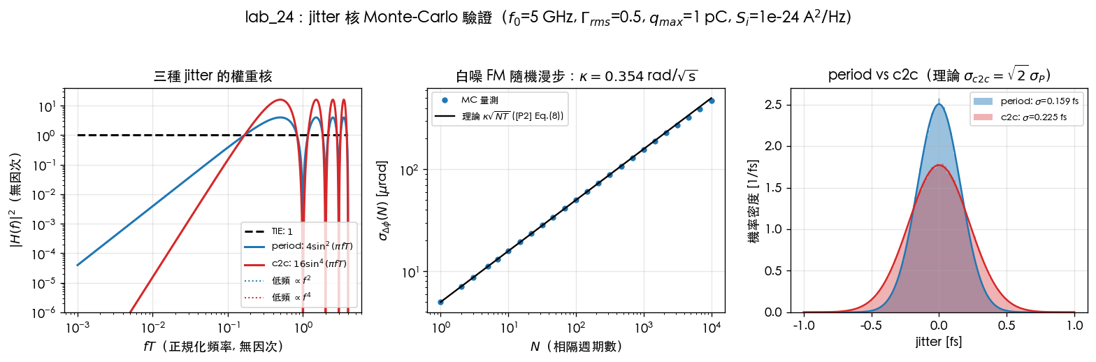
Full script: simulations/lab_24_jitter_kernels.py (run with PYTHONPATH=. python simulations/lab_24_jitter_kernels.py). The simulation has five parts, all using the canonical parameters:

Parameter	Value	Unit	Notes
$f_0$ / $T$	5 GHz / 200 ps	Hz / s	Carrier
$q_{max}$	1	pC	Node charge swing
$S_i$	$10^{-24}$	A²/Hz	One-sided white current-noise PSD
$\Gamma(\theta)$	$-\sqrt2\times0.5\,\sin\theta$	—	rms exactly the representative value $\Gamma_{rms}=0.5$ (reuse gamma_lc_ideal)
$\kappa$	0.3536	rad/$\sqrt{\text{s}}$	$=(\Gamma_{rms}/q_{max})\sqrt{S_i/2}$, $\kappa^2=0.125$ rad²/s
Sampling	32 points/cycle × 2×10⁵ cycles (Part 1); 2×10⁶ cycles (Part 2)	—	Part 2's per-cycle increments $\mathcal{N}(0,\kappa^2T)$ are justified by Part 1
$b_3$ (Part 5)	$6.333\times10^3$	rad²·Hz²	flicker-FM level so that $f_{1/f^3}=b_3/b_2=1$ MHz; record $2^{24}$ periods ⇒ $f_l=298$ Hz

Part 1 — not an abstract random walk, but the mechanism of [P1] Eq.(11): finely sampled white noise current → ISF weighting → cumulative integration → per-cycle phase increment. Verifies that the increment standard deviation $=\kappa\sqrt T$ and that adjacent cycles are uncorrelated:

i_n   = white_noise(n, psd=SI, fs=fs, rng=RNG)          # one-sided PSD = S_i
gamma = np.sqrt(2.0) * GRMS * gamma_lc_ideal(W0 * t)    # rms = 0.5
phi   = np.concatenate(([0.0], np.cumsum(gamma * i_n * dt / QMAX)))
d1    = np.diff(phi[::n_per])                           # per-cycle phase increment
print(f"{rms(d1):.4e}")        # -> 5.0051e-06 rad (theory kappa*sqrt(T)=5.0000e-06)
print(f"{ratio:.3f}")          # -> 1.001
print(f"{corr1:+.4f}")         # -> -0.0012 (adjacent-cycle increments uncorrelated)

Part 2 — measure the three jitters directly in the time domain (a random walk of 2×10⁶ cycles; middle and right columns of the figure):

# N-period phase jitter: rms(phi[N:]-phi[:-N]) vs theory kappa*sqrt(N*T)
# N=1   ratio MC/theory  # -> 0.999
# N=10  ratio            # -> 0.999
# N=100 ratio            # -> 1.001
# period jitter [fs]     # -> 0.1590 fs (theory 0.1592 fs, ratio 0.999)
# cycle-to-cycle [fs]    # -> 0.2248 fs (theory sqrt(2)*sigma_P=0.2251 fs, ratio 0.999)

Part 3 — kernel integral = closed form (numerical cross-check), together with the reconciliation across the three bookkeepings:

S_phi = 2 * KAPPA**2 / (2*np.pi*f)**2                   # white-FM one-sided spectrum
num   = trapz(S_phi * 4*np.sin(np.pi*f*N*T)**2, f) + tail
print(f"{num / (KAPPA**2 * N * T):.4f}")
# -> 1.0000 white noise N=1 (N=10 also 1.0000)
# -> 1.0000 c2c 16sin^4 kernel vs 2*kappa^2*T
# -> 1.0000 flicker numerical integral vs the Step 5 closed form with log
# -> 0.1592 / 0.1592 / 0.1592 fs (one-sided / two-sided / L bookkeeping, all three equal)
# -> -145.0 dBc/Hz (same S_phi, time-domain /2-convention SSB)
# -> -148.0 dBc/Hz ([P1] Eq.(21) /4 convention)

Part 4 — the canonical Example C spectrum ($-100$ dBc/Hz@1 MHz, $1/f^2$), tying the site's three numbers together:

sigma_t, sigma_phi = integrate_rms_jitter(fgrid, L, f0=5e9, fmin=1e6, fmax=100e6)
print(f"{sigma_t*1e15:.1f} fs")     # -> 447.9 fs TIE (Example C, lower-limit dominated)
print(f"{np.sqrt(b2*T**3/2)*1e15:.2f} fs")   # -> 28.28 fs period-jitter closed form
print(f"{kappa_c:.2f}")             # -> 62.83 rad/sqrt(s) (=2π·1MHz·√L_lin; κ_C√T/ω0 also = 28.28 fs)
print(f"{sigma_c3*1e15:.1f} fs")    # -> 27.6 fs Example C3's value truncated to 10^3–10^10 Hz

Part 5 — two-regime growth (white + flicker FM composed; corresponds to Step 5b and [P2] Fig.16): both noise classes are synthesized as per-period phase increments — white increments $\mathcal{N}(0,\kappa^2T)$ (justified by Part 1) plus flicker increments (flicker_noise spectral shaping, level calibrated by Welch) — over $2^{24}$ periods, with $\sigma(\Delta t)$ spanning 5 decades:

b2      = KAPPA2 / (2*np.pi**2); b3 = b2 * 1e6        # target f_{1/f^3} = 1 MHz
k_flick = 2*np.pi**2 * b3 * T**2 * fs                 # so that S_d(f) = 4pi^2 b3 T^2 / f
d_fl    = flicker_noise(n_periods, fs=fs, k_flicker=k_flick, rng=RNG)
d_w     = RNG.normal(0.0, KAPPA*np.sqrt(T), n_periods)
phi     = np.concatenate(([0.0], np.cumsum(d_w + d_fl)))
sig_t   = np.array([rms(phi[N:] - phi[:-N]) for N in Ns]) / W0   # [s]

# flicker level calibration S_d*f  # -> 1.000e-14 rad^2 (nominal also 1.000e-14)
# b3 / f_{1/f^3}                   # -> 6.333e+03 rad^2*Hz^2 / 1.000e+06 Hz
# fitted slope, white region (N≤32)     # -> 0.519 (theory 0.5; exact curve over same window 0.520)
# fitted slope, flicker region (N≥3200) # -> 0.909 (clean ζΔt would be 1.0; exact over same window 0.911)
# corner: MC fit-line intersection  # -> 4.31e-08 s (216 periods)
# corner: self-consistent theory    # -> 4.89e-08 s (245 periods; MC/theory = 0.88)
# identity dt_c·f_{1/f^3}           # -> 0.0489 (= 1/(2×bracket), bracket = 10.22)
# bin sum vs log form (N=10⁴)       # -> 1.089 (f_l=1/T_rec); 0.984 (half-bin correction f_l/2)
# hardware f_l=1 Hz local slope     # -> 0.967 (Δt=1e-7 s; the paper's clean slope-1 fit is justified)
# [P2] osc-12 corner                # -> 6.11e-08 s (171 periods @2.8 GHz)
# implied f_{1/f^3}                 # -> 5.21e+05 Hz (f_l=1 Hz, bracket=15.7)

(Where the 9% bin-sum vs log-form difference comes from: the log closed form takes $f_l=1/T_{rec}$ as the lower limit of a continuous integral, while the first bin of the discrete FFT spectrum actually collects the power of $[f_l/2,\,3f_l/2]$ — replacing $f_l$ by the half-bin-corrected $f_l/2$ moves the ratio to 0.984. The log's sluggishness once more: half a bin moves only 9%.)

How to read the figure: the left column shows the three kernels (log-log); you can directly see the low-frequency behavior — TIE flat, period $\propto f^2$, c2c $\propto f^4$ — and the peak values 4/16. The middle column shows the MC $\sigma_{\Delta\phi}(N)$ landing on the $\kappa\sqrt{NT}$ theory line (slope 1/2, spanning 4 decades). The right column shows the period and c2c histograms: Gaussian, and $\sigma_{c2c}=\sqrt2\,\sigma_P$. This is a pedagogical simulation (single white noise source, linear phase accumulation), not transistor-level.

Reconciliation with Example C3 / Example D: the 27.6 fs of worked_examples Example C3 = the closed-form 28.28 fs with the tail above $10^{10}$ Hz cut off (there the kernel averages 2 and the $1/f^2$ spectrum still contributes ~5% of the variance); the 5.6 fs of psd_phase_noise_jitter Example D is the same kernel integrated only over the 1–100 MHz band. Same set of formulas, same prefactor $1/\omega_0^2$ — all three numbers check out.

Applicability and failure conditions

Condition	When it holds	When it fails
Small jitter: $\sigma_t\ll T$, $\lvert\dot\phi\rvert\ll\omega_0$	first-order edge↔phase mapping (Step 1)	cycle slips, strong injection, large AM-PM
Frequency noise $\nu=\dot\phi$ stationary	kernel formulas remain rigorous for random-walk $\phi$ (Route B)	deterministic drift (temperature, aging) — detrend first, then apply the kernels
$1/f^2$ dominates near $f\sim1/(2NT)$	white-noise closed form $\kappa^2NT$, the $\sqrt2$ relation	flicker corner above $\sim1/(2\pi NT)$: use the Step 5 log formula; the $\sqrt2$ check fails
Flicker closed form: $2\pi NTf_l\ll1$	log formula accurate to $O((2\pi NTf_l)^2)$	long delays / high cutoffs: integrate numerically
TIE with an explicit band $[f_1,f_2]$	numbers are reproducible	free-running oscillator diverges as $f_1\to0$; meaningless without a stated band
Gaussian RJ	$\sigma$ fully describes the distribution (usable for BER extrapolation)	spurs/DJ: the variance formulas still hold, but the distribution is non-Gaussian; BER needs an RJ/DJ decomposition
Two-regime composition: white and flicker statistically independent	$\sigma^2$ add, $\Delta t_c=\kappa^2/\zeta^2$ (Step 5b)	supply/substrate hitting several stages at once (correlated sources): the cross term is nonzero and [P2] Eq.(9)'s "standard deviations add" takes over
Free-running (open-loop)	unbounded two-regime growth	inside a locked PLL: below the loop BW the phase is pulled back, $\sigma$ flattens at long $\Delta t$; a Fig.16-type curve only holds within the loop time constant
Measurement floor subtracted	$\sigma_{\Delta T,\text{eff}}=\sqrt{\sigma_{\Delta T,\text{meas}}^2-\sigma_{\Delta T,\text{min}}^2}$ ([P2] Eq.(39), p.801)	short-$\Delta t$ end swamped by trigger jitter: the white segment looks flattened; subtract the floor before fitting $\kappa$

Corresponding papers / equations

• $\phi(t)=\frac{1}{q_{max}}\int\Gamma i_n\,d\tau$: [P1] Eq.(11), p.182.
• $\sigma_{\Delta\phi}=\kappa\sqrt{\Delta t}$ (phase-jitter random walk): [P2] Eq.(8), p.792; $\kappa=(\Gamma_{rms}/q_{max})\sqrt{S_i/2}$ (no $\omega_0$): [P2] Eq.(11)/(12), p.793 (all verified); phase↔time jitter conversion $\sigma_{\Delta\phi}=2\pi\sigma_{\Delta t}/T$: [P2] Eq.(10), p.793.
• Correlated (1/f) noise, $\sigma\propto\Delta t$: [P2] Eq.(9), p.792 and Fig. 4 (the definition of $\zeta$: "where $\zeta$ is another proportionality constant", verified).
• Two-regime measurement and fits: [P2] Fig.16, p.802 (caption and the $\kappa=6.18\text{e-}9\ \text{sec}^{0.5}$, $\zeta=2.5\text{e}5$ annotations verified verbatim against the rendered page; the missing minus sign in $\zeta$'s printed exponent is the erratum discussed in Section 5b.1); best fit vs the Eq.(12)/(35) theory values $6.18/5.95/6.07\times10^{-9}\sqrt{\text{s}}$: p.801; slope-1 attribution to device 1/f: p.801 and the end of Section VI, pp.797–798; measurement-floor subtraction: Eq.(39), p.801.
• jitter ← phase spectrum (autocorrelation + Khinchin route): [P2] Eq.(46)–(49), p.803 (Appendix A in full, Eq.(40)–(51), starts in the right column of p.802 and ends in the left column of p.803; verbatim transcription and factor-by-factor reconciliation in this page's "Paper-native derivation" section); white-noise special case $\kappa$←$\mathcal{L}$: Eq.(50), p.803; cycle-to-cycle "based on (8)": Eq.(51), p.803 (these three equations verified verbatim in v5 (p.803 rendering): Eq.(49) $\sigma^2_{\Delta\phi}=\tfrac{8}{\omega_0^2}\int_0^\infty S_\phi\sin^2(\pi f\tau)df$ (with $S_\phi$ per Eq.(48) a two-sided spectrum, hence = this page's one-sided $4\sin^2$ kernel); Eq.(50) $\kappa=\tfrac{\Delta f}{f_0}\cdot10^{-\mathcal{L}\{\Delta f\}/20}$ — the minus sign in the exponent means the paper reads $\mathcal{L}$ as "dB below the carrier" (a positive number); with signed dBc values one should read $10^{\mathcal{L}/20}=\sqrt{\mathcal{L}_{lin}}$. Numerical interlock: $-100$ dBc/Hz, $\Delta f=1$ MHz, $f_0=5$ GHz → $\kappa_t=2.0\times10^{-9}\ \sqrt{\text{s}}$, fully consistent with Section 6 of this page ✓; Eq.(51) $\sigma_{CTC}=\tfrac{f}{f_0^{1.5}}\cdot10^{-\mathcal{L}\{\Delta f\}/20}$ (as printed — the numerator reads $f$; the dimensions of Eq.(50)×$\sqrt T$ show it should read the offset frequency $\Delta f$, the $\Delta$ being a printing omission, see A.2 of the "Paper-native derivation" section) — the printed equation has no $\sqrt2$: its $\sigma_{CTC}=\kappa\sqrt{T}$ is "the accumulation over one period" (i.e., this page's $\sigma_P$); with the "adjacent-period difference" definition (this page's $16\sin^4$ kernel) multiply by another $\sqrt2$. Both definitions coexist in the literature; this page names them separately.)
• SSB $/4$ convention: [P1] Eq.(21), p.185 ($-148$ dBc/Hz); time-domain $/2$ convention $-145$ dBc/Hz: the factor-of-2 note in conventions Section 3.
• Operational versions of the kernels and Example D: psd_phase_noise_jitter; Example C3: worked_examples (its TODO is closed by this page).
• Figures: jitter_kernels_mc.png, jitter_two_regime.png (both lab_24).

Key takeaways

• One convention all the way: one-sided $S_\phi$ (rad²/Hz), $\int_0^\infty$, prefactor $1/\omega_0^2$. The "$2/\omega_0^2$" version belongs to the two-sided-spectrum or $\mathcal{L}$ bookkeeping — switching bookkeeping means switching the entire formula.
• Three jitters = 0th/1st/2nd-order differences of $\phi$; kernels $=1$, $4\sin^2(\pi fNT)$, $16\sin^4(\pi fT)$. Every 2 has a pedigree: the 2 from the variance of a difference × the 2 from the half-angle identity (squared again to give 16).
• Rigorous validity of the kernel formulas only requires stationary frequency noise (boxcar derivation); random-walk phase is covered.
• Punchline: inserting white FM into kernel (b) gives exactly $\sigma_{\Delta\phi}^2(N)=\kappa^2NT$ — the frequency-domain kernel picture and the time-domain random walk of [P2] Eq.(8)/(11)/(12) are one and the same thing; MC ratios 0.999–1.001.
• $\sigma_{c2c}=\sqrt2\,\sigma_P$ (white noise only); $\kappa=2\pi\Delta f\sqrt{\mathcal{L}_{\text{lin}}}$ (remember to use the $/2$-convention $\mathcal{L}$: $-145$, not $-148$).
• Flicker: $\sigma_{\Delta\phi}^2(N)=4\pi^2b_3(NT)^2[\tfrac32-\gamma-\ln(2\pi NTf_l)]$, logarithmically dependent on the low-frequency cutoff; a report must include $f_l$; the growth law is approximately $\propto N$ (the slope-1 segment of [P2] Eq.(9)).
• The two-regime whole picture ([P2] Fig.16): $\sigma(\Delta t)=\sqrt{\kappa^2\Delta t+\zeta^2\Delta t^2}$ (independent ⇒ variances add), corner $\Delta t_c=\kappa^2/\zeta^2$; time↔frequency mapping $\Delta t_c=1/(2[\cdot]f_{1/f^3})$ with $[\cdot]\approx10$–$16$ ⇒ 20–30× shorter than $1/f_{1/f^3}$; osc-12: 61 ns (171 periods), canonical: 49 ns (245 periods); MC slopes 0.519/0.909 = the exact curve's 0.520/0.911 (the deviations from 0.5/1.0 are log physics).
• Canonical numbers: representative oscillator $\kappa^2=0.125$ rad²/s, $\sigma_P=0.159$ fs, $\sigma_{c2c}=0.225$ fs, $\mathcal{L}(1\text{MHz})=-145/-148$ dBc/Hz ($/2$, $/4$ conventions); Example C spectrum: TIE(1–100 MHz)$=447.9$ fs, period-jitter closed form $28.28$ fs (Example C3's 27.6 fs is the band-truncated value).

Further reading

• Operational versions of the kernels, the four-step $\mathcal{L}\to S_\phi\to\sigma_t$ chain, and Examples C/D: psd_phase_noise_jitter
• Difference kernels of the same family (gated average + adjacent difference): allan_variance
• The ISF origin of $\kappa$ and the ring-oscillator $\Gamma_{rms}$: paper_002 deep dive
• White noise → $1/f^2$ phase spectrum (full discussion of the $/2$ vs $/4$ conventions): white_noise_to_phase_noise
• What the spectrum of a random-walk phase looks like (Lorentzian line shape): lorentzian_linewidth
• Impact of jitter on SerDes BER: serdes_clocking_connection