LTI vs LTV — an Oscillator's Noise Sensitivity Is Periodically Time-Varying

β: This English translation is in beta — the Traditional-Chinese original is the authoritative version.

Prerequisites: oscillator_phase · phase_vs_amplitude_noise | Next: From impulse to phase shift — the derivation

Signals-and-systems courses teach us to describe linear systems with an impulse response $h(t)$ and convolution. But that is the LTI (Linear Time-Invariant) story. The single most important insight of Hajimiri–Lee in [P1] is:

An oscillator's phase response to noise is not LTI — it is LTV (Linear Time-Variant).

This page spells out how LTI and LTV differ, why an oscillator is necessarily LTV, and why this difference is exactly the reason the ISF (Impulse Sensitivity Function) exists.

Physical intuition (conclusion first): an LTI system "does not care what time it is" — the same impulse applied today or tomorrow produces exactly the same response shape, merely shifted in time. An oscillator is not like that: because its state keeps rotating around the limit cycle, the same noise current injected at the peak versus at a zero crossing produces completely different phase shifts. The system's sensitivity to the input itself varies periodically with time (with the injection phase) — this is "periodically time-varying sensitivity", and packaging it into a $2\pi$-periodic, dimensionless function gives the ISF $\Gamma(\omega_0\tau)$.

1. Review: the LTI $h(t-\tau)$

A linear time-invariant system has two properties: linearity (superposition holds) and time invariance (delay the input by $\Delta$ and the output is simply delayed by $\Delta$, shape unchanged). The consequence of time invariance is that the impulse response depends only on the time difference $t-\tau$:

$$y(t)=\int_{-\infty}^{\infty}h(t-\tau)\,x(\tau)\,d\tau\qquad\text{(LTI convolution)}.$$

• Why only $t-\tau$: inject a unit impulse at $\tau_1$ and you get $h(t-\tau_1)$; inject at $\tau_2$ and you get $h(t-\tau_2)$ — the same shape, merely shifted. The system does not care about "the absolute time $\tau$", only about "how long ago".
• Unit check: the dimension of the convolution kernel $h$ is set by output/input; the point here is "shape invariance", not the numerical value.
• This is the undergraduate story: RLC filters, small-signal amplifier equivalents — as long as the operating point is fixed, they are LTI.

2. The oscillator: the impulse response becomes $h(t,\tau)$ — one extra independent variable

An oscillator has no fixed operating point — its state keeps moving along the limit cycle (see oscillator_phase). So "how sensitive the system is to a perturbation right now" changes with the state (that is, with the injection phase $\omega_0\tau$). The impulse response therefore depends on two times at once:

$$\boxed{\;h_\phi(t,\tau)\neq h_\phi(t-\tau)\;}\qquad\text{(LTV: depends on the absolute injection time }\tau\text{, not only }t-\tau\text{)}.$$

The excess-phase impulse response [P1] writes down is exactly of this form ([P1] Eq.(10), p.182):

$$h_\phi(t,\tau)=\frac{\Gamma(\omega_0\tau)}{q_{max}}\,u(t-\tau).$$

Unpacking it, the two independent variables of the LTV response map neatly onto the two factors, each with a clear meaning:

• Step height $\dfrac{\Gamma(\omega_0\tau)}{q_{max}}$: depends only on the injection phase $\omega_0\tau$. This is the "time-varying" part — the same-size impulse jumps by a different height at a different injection phase.

• Time shape $u(t-\tau)$: a unit step, depending only on $t-\tau$. It encodes "once a phase shift occurs it is retained permanently" (phase has no restoring force; see phase_vs_amplitude_noise).

• Unit check / dimension: $\Gamma$ is dimensionless, $q_{max}$ has units of C, $u$ is dimensionless, so $h_\phi$ has units of $\mathrm{C^{-1}}$; convolving with a current (A), $\int h_\phi\,i\,d\tau$ gives $\mathrm{C^{-1}\cdot A\cdot s}=\mathrm{C^{-1}\cdot C}=$ dimensionless = rad ✓.

• Why $\Gamma(\omega_0\tau)$ and not $\Gamma(\tau)$: the sensitivity varies periodically with the "waveform phase", with period $2\pi$ (every lap around the limit cycle returns to the same sensitivity). So the argument of $\Gamma$ is the phase $\omega_0\tau$, and $\Gamma$ is a $2\pi$-periodic function — this is "periodically time-varying sensitivity".

3. Why the same impulse produces different phase shifts at different positions

Plug the step height of Step 2 into the operational ISF definition (the impulse limit of [P1] Eq.(11)):

$$\Delta\phi(\tau)=\frac{\Gamma(\omega_0\tau)}{q_{max}}\,\Delta q.$$

Fix $\Delta q$ and sweep the injection phase $\theta=\omega_0\tau$: $\Delta\phi$ rises and falls following the shape of $\Gamma(\theta)$. For an ideal LC, $\Gamma(\theta)=-\sin\theta$:

Injection phase $\theta$	Waveform position	$\Gamma(\theta)=-\sin\theta$	Result
$0$	Peak (0 slope)	$0$	$\Delta\phi=0$, pure amplitude change
$\pi/2$	Falling zero crossing (most negative slope)	$-1$	$\vert \Delta\phi\vert$ maximum
$\pi$	Trough (0 slope)	$0$	$\Delta\phi=0$, pure amplitude change
$3\pi/2$	Rising zero crossing (most positive slope)	$+1$	$\vert \Delta\phi\vert$ maximum, opposite sign

• Physical reason (continuing Step 4 of oscillator_phase): the size of the phase shift is set by the component of the voltage jump projected onto the tangential direction of the limit cycle. At a zero crossing the state velocity (tangent) lies exactly along the voltage axis, so a fixed $\Delta V$ turns almost entirely into tangential displacement → maximum $\Delta\phi$; at the peak the tangent is perpendicular to the voltage axis, so $\Delta V$ is almost entirely radial (pure amplitude) → $\Delta\phi\approx 0$. The tangential component is $\propto\sin\theta$, hence $\Gamma(\theta)=-\sin\theta$ for a sinusoid.
• This is the fingerprint of LTV: if the oscillator were LTI, $\Delta\phi$ would be independent of $\tau$ (only $t-\tau$ would matter) — but in reality $\Delta\phi(\tau)$ rises and falls periodically. The sensitivity itself varies with time = time-variant.

Putting LTI and LTV side by side makes it clearest:

	LTI	LTV (oscillator phase)
Impulse response	$h(t-\tau)$ (time difference only)	$h_\phi(t,\tau)=\dfrac{\Gamma(\omega_0\tau)}{q_{max}}u(t-\tau)$
Changing the injection time $\tau$	Shape unchanged, only shifted	Step height changes with $\omega_0\tau$
Sensitivity	Independent of absolute time	$2\pi$-periodically time-varying (= ISF)
Convolution	$\int h(t-\tau)x\,d\tau$	$\dfrac{1}{q_{max}}\displaystyle\int_{-\infty}^{t}\Gamma(\omega_0\tau)i_n(\tau)\,d\tau$

The LTV convolution in the bottom-right cell is [P1] Eq.(11), p.182 — the next chapter's convolution_derivation uses it to superpose an arbitrary noise current into $\phi(t)$.

4. Side-by-side figure: LTI shape fixed vs LTV step height varying with phase

The upper half of the figure below is the impulse response of an LTI system (a simple first-order decay): injecting at $\tau=0.3,\,0.9,\,1.5$ yields the same shape, merely shifted. The lower half is the oscillator's LTV phase response $h_\phi(t,\tau)$: at different injection phases $\tau$, the step height $\Gamma(\omega_0\tau)=-\sin(2\pi\tau)$ changes accordingly (it even flips sign).

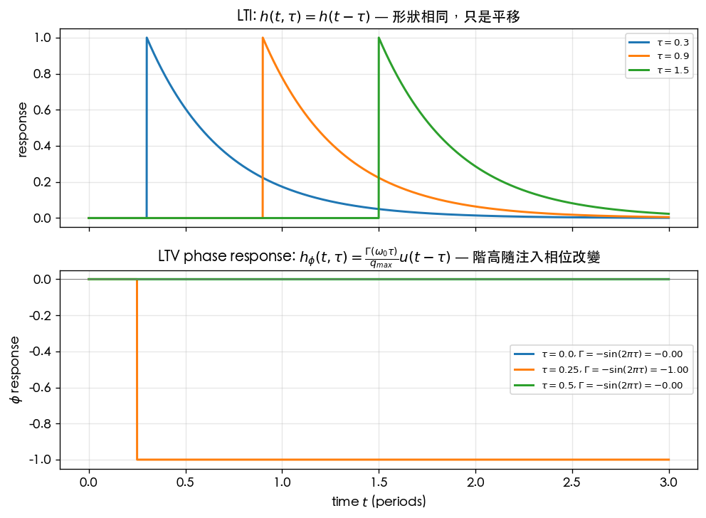
How to read this figure:

• Upper half (LTI): the three curves, overlaid, have exactly the same shape — only the starting points are shifted: "the system ignores absolute time".
• Lower half (LTV): all three are steps ($u(t-\tau)$, retained permanently), but the step heights differ: at $\tau=0$, $\Gamma=-\sin 0=0$ (injected at the peak: 0 step height, no phase shift); at $\tau=0.25$, $\Gamma=-\sin(\pi/2)=-1$ (injected at the zero crossing: maximum step height, negative); at $\tau=0.5$, $\Gamma=-\sin(\pi)=0$ (injected at the trough: 0 step height).
• Message: the LTV "shape" is fixed (always a step, because phase has no restoring force), but the "strength" is periodically time-varying — and that is exactly the ISF.

The next figure sweeps the step height continuously over the injection phase (the phase sweep of lab_04) — effectively drawing that table column as a continuous curve; the numerics nearly coincide with the theoretical $-\sin\theta$:

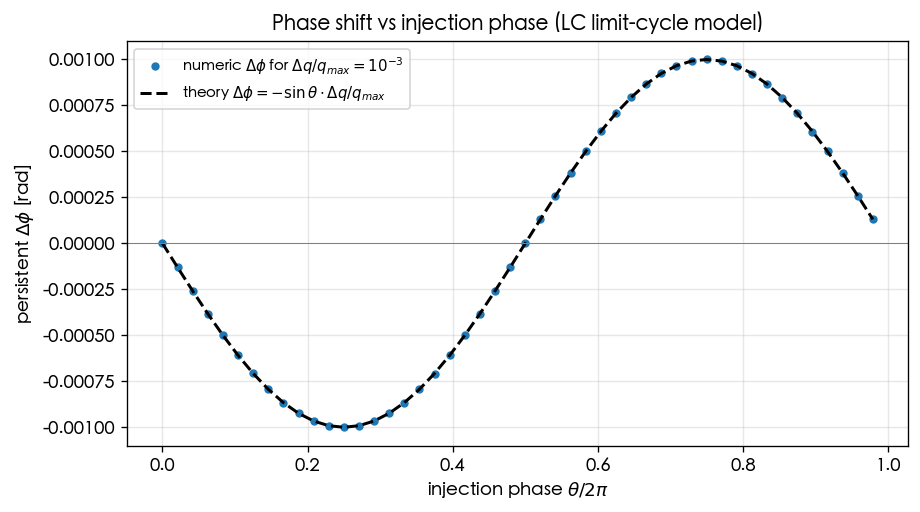
How to read this figure: the horizontal axis is the injection phase $\theta/2\pi$ (one period); the vertical axis is the permanently retained $\Delta\phi$ after injection (fixed $\Delta q/q_{max}=10^{-3}$). Blue dots are the numerical simulation; the black dashed line is $\Delta\phi=-\sin\theta\cdot\Delta q/q_{max}$. $\Delta\phi$ rising and falling periodically with the injection phase is LTV made visible; it is proportional to the ISF, so this sweep is essentially "a measured $\Gamma(\theta)$".

Generating both figures with the real functions

Both figures are produced by simulations/lab_04_impulse_sweep.py. The LTV comparison figure sets the step heights with the analytic ISF $\Gamma(\theta)=-\sin(2\pi f_0\tau)$; the phase-sweep figure uses extract_isf_by_injection() to actually inject a small charge into the limit-cycle model and measure the persistent phase shift:

import numpy as np
from oscillator_models import extract_isf_by_injection

# (1) LTV comparison: step height = ISF(injection phase); time shape is always u(t - tau)
f0 = 1.0
for tau in [0.0, 0.25, 0.5]:
    gamma = -np.sin(2 * np.pi * f0 * tau)   # ISF at injection phase
    # h_phi(t, tau) = gamma * u(t - tau)    -> step height changes with tau; shape (a step) does not

# (2) Phase sweep: numerically extract the ISF, compare with the analytic -sin(theta)
theta, g_num, g_ana = extract_isf_by_injection(
    f0=1.0, fs=8000.0, n_inject_periods=6, settle_periods=4,
    dq_over_qmax=1e-3, n_points=48, mu=0.3)
# g_num ≈ g_ana = -sin(theta); maximum error about 0.001

Full script: simulations/lab_04_impulse_sweep.py (core model: extract_isf_by_injection and simulate_lc in simulations/common/oscillator_models.py).

Parameter table:

Parameter	Symbol	LTV comparison figure	Phase-sweep figure	Unit
Oscillation frequency	$f_0$	1.0 (normalized)	1.0 (normalized)	Hz
Sampling rate	$f_s$	2000	8000	Hz
Injection phase	$\tau$	$\{0,\,0.25,\,0.5\}$ periods	48-point sweep over one period	—
Relative injected charge	$\Delta q/q_{max}$	(illustrative step height)	$10^{-3}$ (small-signal)	—
Settling periods	—	—	4	—
Amplitude-restoring strength	$\mu$	— (analytic step height)	0.3	—

Toy-model warning: both figures are pedagogical toy models, not transistor-level. The LTV figure sets the step heights with the analytic $-\sin$; the sweep figure uses a normalized 2-D limit-cycle model to reproduce the mechanism of "periodically time-varying sensitivity" — the numbers are for teaching. Corresponds to [P1] Eqs.(10),(11), Sec. III, and Fig. 4.

5. Why LTV is unavoidable — where the LTI model goes wrong

Historically, treating oscillator noise as LTI (e.g., simply multiplying the noise by the tank transfer function) misses two things that only LTV/ISF can capture:

1. Frequency translation: because the sensitivity $\Gamma(\omega_0\tau)$ is itself periodic (containing harmonics of $\omega_0$), it mixes noise near $0,\,\omega_0,\,2\omega_0,\dots$ down next to the carrier. LTI does not mix, and therefore cannot explain why device noise both at DC and at $n\omega_0$ shows up in close-in phase noise. This is described by the Fourier coefficients $c_n$ of the ISF ([P1] Eq.(12)–(13), p.183).
2. $1/f$ upconversion into $1/f^3$: the device's low-frequency $1/f$ noise reaches the vicinity of the carrier through the ISF's DC coefficient $c_0$ ([P1] Eq.(23)); a purely LTI view cannot explain it. Waveform symmetry → small $c_0$ → suppressed $1/f^3$ corner ([P1] Eq.(24)).

In other words, LTV is not a gratuitous complication — the oscillator is physically time-varying; forcing an LTI model misses mixing and $1/f$ upconversion, two real phenomena, already at the qualitative level.

Numerical example (building intuition)

LTV version of Example A: $q_{max}=1$ pC, $\Delta q=1$ fC, $f_0=5$ GHz; compare injecting at a zero crossing ($\Gamma=-1$) with injecting at the peak ($\Gamma=0$).

Zero crossing ($\theta=\pi/2$, $\Gamma=-\sin(\pi/2)=-1$):

$$|\Delta\phi|=\frac{|\Gamma|\,\Delta q}{q_{max}}=\frac{1\times(1\times10^{-15})}{1\times10^{-12}}=1\times10^{-3}\ \text{rad}\ \Rightarrow\ \Delta t=\frac{10^{-3}}{2\pi\times5\times10^{9}}\approx31.8\ \text{fs}.$$

Peak ($\theta=0$, $\Gamma=0$): $\Delta\phi=0$ rad, $\Delta t=0$ fs.

• Dimension check: $[\text{rad}]/[\text{rad/s}]=[\text{s}]$ ✓.
• Feel for the numbers: the same 1 fC — because the sensitivity is periodically time-varying, a $90^\circ$ change in injection phase takes the phase shift from 31.8 fs down to 0. That phase-dependent ratio, written down as a function, is the ISF — the entire spirit of LTV in one sentence.

Applicability and failure conditions

Condition	When it holds	What happens when it fails
Small signal (linearization)	Response is linear in $\Delta q$; $h_\phi(t,\tau)$ is well defined	Large injection → genuinely nonlinear; even LTV linear superposition is insufficient
A steady-state periodic orbit exists	$\Gamma$ is a well-defined $2\pi$-periodic function	Before start-up / during chirp / FM, $\Gamma$ no longer has a fixed period
The correct $\Gamma$ is known	The LTV convolution predicts $\phi(t)$	$\Gamma$ must be extracted by transient/adjoint simulation (see effective_isf)
Phase has no restoring force	Using $u(t-\tau)$ (permanent step) is justified	Under strong injection locking the phase is held by an external force ([P3])

Key takeaways

• LTI: $h(t-\tau)$ — only the time difference matters; changing the injection time merely shifts the response, shape unchanged.
• LTV: $h_\phi(t,\tau)=\dfrac{\Gamma(\omega_0\tau)}{q_{max}}u(t-\tau)$ — the step height varies periodically with the injection phase $\omega_0\tau$; the time shape (a step) is fixed.
• An oscillator is necessarily LTV: the state moves along the limit cycle → sensitivity varies with phase → same impulse, different position → different $\Delta\phi$.
• The ISF $\Gamma(\omega_0\tau)$ is, in essence, "periodically time-varying sensitivity"; for the ideal LC it is $-\sin\theta$.
• Only LTV explains frequency translation ($c_n$ mixing) and $1/f\to1/f^3$ upconversion ($c_0$); LTI misses both.
• Example A: 1 fC injected at a zero crossing → 31.8 fs; at the peak → 0 fs (a direct consequence of periodically time-varying sensitivity).
• Sources: [P1] Eq.(10), Eq.(11), Sec. III; numbers and figures from lab_04.

Further reading

• The geometric starting point: oscillator_phase
• Why phase accumulates while amplitude decays: phase_vs_amplitude_noise
• Turning LTV into the full derivation: From impulse to phase shift — the derivation
• Superposing arbitrary noise with the LTV convolution: convolution_derivation
• $c_n$ mixing and frequency translation: fourier_series_of_isf
• The matching numerical experiment: Numerical Feeling