Fourier Series of the ISF

β: This English translation is in beta — the Traditional-Chinese original is the authoritative version.

Prerequisites: isf_definition ($\Gamma$ is dimensionless and $2\pi$-periodic), impulse_to_phase_shift (the operational definition of $\Gamma$), convolution_derivation (the phase integral for continuous noise).

Hands-on verification: the Fourier-coefficient extraction, reconstruction, and Parseval numerical checks for this page are in lab_05.

The previous chapter impulse_to_phase_shift derived the operational definition of the ISF, $\Delta\phi=\Gamma(\omega_0\tau)\,\Delta q/q_{max}$, and pointed out that $\Gamma$ is a dimensionless, $2\pi$-periodic function. This page answers the next key question:

Given that $\Gamma$ is periodic, once it is expanded as a Fourier series, what physics does each term represent? The answer is the most elegant piece of ISF theory — it spells out exactly which band of device noise the oscillator moves to the vicinity of the carrier. The core result ([P1] Eq.(12), p.183):

$$\Gamma(\omega_0\tau)=\frac{c_0}{2}+\sum_{n=1}^{\infty}c_n\cos(n\omega_0\tau+\theta_n)$$

Physical intuition (conclusion first): an oscillator is a time-varying mixer. Its phase sensitivity to noise, $\Gamma$, varies periodically with the waveform phase — equivalent to multiplying the noise by a "periodic weight" with fundamental $\omega_0$. Multiplying noise by a periodic function is, mathematically, shifting the noise spectrum to $0,\ \omega_0,\ 2\omega_0,\dots$ and summing. So device noise near each $n\omega_0$ is weighted by the $n$-th Fourier coefficient $c_n$ and then down-converted to the carrier vicinity as phase noise. The $c_0$ (DC) term is especially important: it moves the 1/f flicker noise near DC straight up, producing the close-in $1/f^3$ phase noise.

Step 1: why $\Gamma$ can be expanded as a Fourier series

$\Gamma(\omega_0\tau)$ describes "how far the phase is pushed by a kick at a given point of the waveform". The oscillator sits in periodic steady state (the output waveform repeats every $T=1/f_0$), so "kicking at phase $x$" and "kicking at phase $x+2\pi$" have exactly the same effect. In other words $\Gamma$ is $2\pi$-periodic in its argument $x\equiv\omega_0\tau$:

$$\Gamma(x+2\pi)=\Gamma(x).$$

• Math used: any $2\pi$-periodic function that is square-integrable over one period ($\int_0^{2\pi}|\Gamma|^2dx<\infty$) admits a Fourier series (Dirichlet conditions). Real ISFs are continuous and piecewise smooth, so the conditions are easily satisfied.
• Physical basis: the periodicity comes from the oscillator's limit cycle — in steady state the state point goes around the cycle once per period, and the sensitivity depends only on the "position on the cycle (phase)", not on "which lap".
• Unit check: $x=\omega_0\tau$ is $[\text{rad/s}]\cdot[\text{s}]=[\text{rad}]$ ✓, dimensionless; $\Gamma$ itself is dimensionless, and so are $c_0,c_n$ (see notation).

Step 2: write the standard Fourier expansion (cos/sin form)

First write the familiar real cos/sin Fourier series, then merge it into the amplitude–phase form of [P1]. For a $2\pi$-periodic function:

$$\Gamma(x)=\frac{a_0}{2}+\sum_{n=1}^{\infty}\big[a_n\cos(nx)+b_n\sin(nx)\big],$$

with the coefficients obtained by inner products (projections) over one period:

$$a_0=\frac{1}{\pi}\int_0^{2\pi}\Gamma(x)\,dx,\qquad a_n=\frac{1}{\pi}\int_0^{2\pi}\Gamma(x)\cos(nx)\,dx,\qquad b_n=\frac{1}{\pi}\int_0^{2\pi}\Gamma(x)\sin(nx)\,dx.$$

• Math used: $\{\cos(nx),\sin(nx)\}$ are orthogonal on $[0,2\pi]$, $\int_0^{2\pi}\cos(mx)\cos(nx)\,dx=\pi\,\delta_{mn}$ ($m,n\ge1$); this orthogonality "sifts" out the corresponding component.
• Watch the $1/\pi$ and the DC factor: $a_0=\frac{1}{\pi}\int_0^{2\pi}\Gamma\,dx$, while the mean (DC value) of $\Gamma$ is $\frac{1}{2\pi}\int_0^{2\pi}\Gamma\,dx=\frac{a_0}{2}$. So the first term of the series must be written $\frac{a_0}{2}$ to equal the true mean. This $1/2$ is not arbitrary; the definition of $c_0$ below inherits it.

Step 3: merge into amplitude–phase form to get $c_n,\theta_n$

Combine the same-frequency pair $a_n\cos(nx)+b_n\sin(nx)$ into a single cosine via the trig identity:

$$a_n\cos(nx)+b_n\sin(nx)=c_n\cos(nx+\theta_n),$$

where

$$c_n=\sqrt{a_n^2+b_n^2},\qquad \theta_n=\operatorname{atan2}(-b_n,\,a_n).$$

• Math used: $c_n\cos(nx+\theta_n)=c_n\cos\theta_n\cos(nx)-c_n\sin\theta_n\sin(nx)$; matching coefficients gives $a_n=c_n\cos\theta_n$, $b_n=-c_n\sin\theta_n$; inverting yields the expressions above.
• DC correspondence: set $c_0\equiv a_0$ (the DC coefficient), so the constant term $\frac{a_0}{2}=\frac{c_0}{2}$. Substituting gives [P1] Eq.(12):

$$\boxed{\ \Gamma(\omega_0\tau)=\frac{c_0}{2}+\sum_{n=1}^{\infty}c_n\cos(n\omega_0\tau+\theta_n)\ }\qquad[\text{P1] Eq.(12), p.183}$$

• Notation trap (important): $c_0$ is the Fourier coefficient, while the DC value of the ISF is $c_0/2$. This factor is the easiest place to slip when computing the $1/f^3$ corner (Eq.(24)); later chapters will keep reminding you. The a0 returned by this site's Python compute_fourier_coefficients equals this $c_0$ (see Step 8).

Step 4: the physics of $c_0$ — DC, controls $1/f$ upconversion

Substitute the Fourier expansion of the ISF back into the LTV phase response ([P1] Eq.(11)→Eq.(13), p.183):

$$\phi(t)=\frac{1}{q_{max}}\!\left[\frac{c_0}{2}\!\int_{-\infty}^{t}\!i_n\,d\tau+\sum_{n=1}^{\infty}c_n\!\int_{-\infty}^{t}\!i_n\cos(n\omega_0\tau+\theta_n)\,d\tau\right]\qquad[\text{P1] Eq.(13), p.183}$$

The first term (the $c_0$ term) integrates the noise current directly, without any $\cos(n\omega_0\tau)$ modulation. Meaning:

• The $c_0$ term responds to the DC / very-low-frequency components of the noise current — push the node slowly and the phase drifts slowly.
• Inject a small tone near DC, $i(t)=I_0\cos(\Delta\omega t)$ ($\Delta\omega\ll\omega_0$): only the $c_0$ term responds (the other harmonics are averaged out by $\cos(n\omega_0\tau)$), giving ([P1] Eq.(15), p.183):

$$\phi(t)\approx\frac{I_0\,c_0\sin(\Delta\omega t)}{2q_{max}\,\Delta\omega}.$$

• Why this is called "$1/f$ upconversion": device flicker / $1/f$ noise is concentrated at low frequency (near DC). The $c_0$ term moves (up-converts) this "noise living at baseband" next to the carrier, turning it into close-in phase noise. Later, flicker_noise_upconversion uses this to derive the $1/f^3$ skirt ([P1] Eq.(23),(24)).
• Design implication: the smaller $c_0$, the weaker the flicker upconversion. With $c_0=0$ (a perfectly symmetric waveform), close-in theoretically has no $1/f^3$ contribution. This is the mathematical root of the "waveform symmetry → close-in phase noise" design rule (experimentally supported by [P2] Fig. 17, p.802).

Step 5: the physics of $c_n$ — frequency-translating noise near $n\omega_0$ to the carrier

Look at the $n$-th component of the second term of Eq.(13): it multiplies the noise current by $\cos(n\omega_0\tau+\theta_n)$ and then integrates. Multiplying by $\cos(n\omega_0\tau)$ is, in the frequency domain, shifting the noise spectrum by $\pm n\omega_0$ (modulation theorem). So:

• Device noise near $n\omega_0+\Delta\omega$ (and $n\omega_0-\Delta\omega$) is weighted by $c_n$ and down-converted to $\Delta\omega$, becoming the phase noise at offset $\Delta\omega$ from the carrier.
• Inject a small tone near $n\omega_0$, $i(t)=I_0\cos((n\omega_0+\Delta\omega)t)$, into Eq.(13): only the $n$-th harmonic responds, giving ([P1] Eq.(16)/(17), p.183):

$$\phi(t)\approx\frac{I_0\,c_n\sin(\Delta\omega t)}{2q_{max}\,\Delta\omega}.$$

Explicit algebra: using $\cos A\cos B$ to move noise near $n\omega_0$ to the carrier

The line above is the "result"; now we work the frequency-translation algebra out in full, not just the intuition. Take the $n$-th component of the second term of Eq.(13) and substitute the single tone $i_n(\tau)=I_0\cos((n\omega_0+\Delta\omega)\tau)$:

$$\phi_n(t)=\frac{c_n}{q_{max}}\int_{-\infty}^{t}\cos(n\omega_0\tau+\theta_n)\,I_0\cos\big((n\omega_0+\Delta\omega)\tau\big)\,d\tau .$$

Step (i): product-to-sum. The product of the two cosines uses the identity

$$\cos A\cos B=\tfrac12\big[\cos(A-B)+\cos(A+B)\big],$$

with $A=n\omega_0\tau+\theta_n$, $B=(n\omega_0+\Delta\omega)\tau$; compute the difference and sum frequencies:

$$A-B=\theta_n-\Delta\omega\tau\quad(\text{frequency}\approx\Delta\omega),\qquad A+B=(2n\omega_0+\Delta\omega)\tau+\theta_n\quad(\text{frequency}\approx 2n\omega_0).$$

The integrand becomes two terms:

$$\cos(n\omega_0\tau+\theta_n)\cos\big((n\omega_0+\Delta\omega)\tau\big)=\tfrac12\Big[\cos(\Delta\omega\tau-\theta_n)+\cos\big((2n\omega_0+\Delta\omega)\tau+\theta_n\big)\Big].$$

This line is the core of "frequency translation": noise that originally lived at $n\omega_0+\Delta\omega$, once multiplied by $\cos(n\omega_0\tau)$, has its difference frequency collapse down to $\Delta\omega$ at baseband (moved down), while its sum frequency is pushed to $2n\omega_0$ (higher, useless).

Step (ii): the integrator amplifies only the slow term and averages out the fast one. $\int^t d\tau$ is a low-pass:

$$\int^{t}\cos(\Delta\omega\tau-\theta_n)\,d\tau=\frac{\sin(\Delta\omega t-\theta_n)}{\Delta\omega}\ (\text{slow; small denominator}\Rightarrow\text{amplified, survives}),$$ $$\int^{t}\cos\big((2n\omega_0+\Delta\omega)\tau+\theta_n\big)\,d\tau=\frac{\sin(\cdots)}{2n\omega_0+\Delta\omega}\ (\text{fast; denominator}\approx2n\omega_0\Rightarrow\text{suppressed to negligible}).$$

Step (iii): keep only the slow term.

$$\phi_n(t)\approx\frac{c_n}{q_{max}}\cdot\frac{I_0}{2}\cdot\frac{\sin(\Delta\omega t-\theta_n)}{\Delta\omega}=\frac{I_0\,c_n\sin(\Delta\omega t-\theta_n)}{2q_{max}\,\Delta\omega},$$

Absorbing the fixed phase $\theta_n$ into the origin recovers Eq.(16/17). Conclusion: the $n$-th Fourier coefficient $c_n$ really does take the noise near $n\omega_0$, "multiply it by $\tfrac12 c_n$ and collapse it to $\Delta\omega$" — this is the algebraic proof of frequency translation, matching the mixer picture below. (The same downconversion integral is used again in white_noise_to_phase_noise to accumulate the $1/f^2$ summation.)

• This is exactly the picture of [P1] Fig. 8 (p.183): noise is spread across the bands at $0,\omega_0,2\omega_0,\dots$; the ISF's $c_0,c_1,c_2,\dots$ act like a bank of mixer gains, each folding its band's noise back to the carrier vicinity, all superposing into the final phase-noise sideband.

• Unit/dimension check: in Eq.(15)/(16) the dimensions of $\dfrac{I_0\,c_n}{2q_{max}\,\Delta\omega}$ are $\dfrac{[\text{A}]\cdot(\text{dimensionless})}{[\text{C}]\cdot[\text{rad/s}]} =\dfrac{[\text{A}]}{[\text{C/s}]\cdot[\text{rad}]}=\dfrac{[\text{A}]}{[\text{A}]}\cdot\dfrac{1}{[\text{rad}]^{-1}}$ — after simplification $\phi$ is rad (dimensionless), and $\sin(\Delta\omega t)$ is dimensionless ✓. (Remember $C=\text{A}\cdot\text{s}$.)

Step 6: why close-in ($1/f^3$) is dominated by $c_0$ and the low-order coefficients

Put the two steps above together into one "frequency map":

Where the device noise lives	Via which coefficient	What it becomes next to the carrier
$1/f$ flicker near DC	$c_0/2$	close-in, slope $1/f^3$ (very steep)
White noise near $\omega_0$	$c_1$	$1/f^2$ skirt ($-20$ dB/dec)
White noise at $2\omega_0,3\omega_0,\dots$	$c_2,c_3,\dots$	also folds back, merged into $1/f^2$ (counted via $\sum c_n^2$)

• Why flicker becomes $1/f^3$ through $c_0$: flicker is already $1/f$ (power spectrum $\propto1/\Delta\omega$). The $c_0$ term moves it intact next to the carrier; the phase integrator (the $\int d\tau$ in Eq.(13)) then adds another $1/\Delta\omega^2$ (integration divides by $(j\Delta\omega)$ in frequency, i.e. by $\Delta\omega^2$ in power), $\dfrac{1}{\Delta\omega}\times\dfrac{1}{\Delta\omega^2}=\dfrac{1}{\Delta\omega^3}$ → $1/f^3$.
• Why the higher-order $c_n$ mainly feed $1/f^2$: white noise is flat — flat wherever it is moved — and the integrator only adds $1/\Delta\omega^2$ → $1/f^2$. All harmonic contributions are summarized by a single number, $\sum_{n=0}^\infty c_n^2$, which is exactly the Parseval relation and $\Gamma_{rms}$ of the next page rms_isf.
• The full $1/f^3$ / $1/f^2$ derivations are in flicker_noise_upconversion and white_noise_to_phase_noise respectively.

Step 7: how waveform symmetry nulls certain coefficients

The parity of the Fourier coefficients follows directly from the symmetry of $\Gamma(x)$, giving the designer a knob to "switch off certain upconversions via the waveform shape":

Symmetry of $\Gamma$	Mathematical result	Physical consequence
Even function $\Gamma(-x)=\Gamma(x)$	all $b_n=0$ (pure cos)	$\theta_n\in\{0,\pi\}$, simple phases
Odd function $\Gamma(-x)=-\Gamma(x)$	all $a_n=0$ and $a_0=0$ ⟹ $c_0=0$	no $1/f$ upconversion (the ideal-LC $-\sin$ is of this type)
Half-wave symmetry $\Gamma(x+\pi)=-\Gamma(x)$	even harmonics $c_2=c_4=\dots=0$	noise near $2\omega_0$ does not fold back
DC offset $\cos\theta+\alpha$ (toy gamma_asymmetric)	$c_0=2\alpha\neq0$	$1/f^3$ appears (close-in degrades)

• Example (ideal LC): $\Gamma_{LC}(\theta)=-\sin\theta$ is odd ⟹ $c_0=0$. So the ideal LC has, to first order, no flicker upconversion; it is real-world asymmetry (hard switching, bias asymmetry) that props $c_0$ up.
• Example (half-wave symmetry): differential / push-pull structures make the rising and falling edges mirror images ⟹ $\Gamma(x+\pi)=-\Gamma(x)$ ⟹ the even harmonics are suppressed, and noise at $2\omega_0$ (often supply ripple and second-harmonic distortion) does not fold back to the carrier.
• Note (mechanism of the toy model): the gamma_asymmetric in the table props $c_0$ up in the simplest possible way — adding a DC offset to the whole ISF ($\cos\theta+\alpha$); in real circuits, asymmetric rise/fall transition slopes are a different — and more common — mechanism that likewise makes $c_0\neq0$ and turns on $1/f$ upconversion, but with a different waveform shape. The toy on this page exists only to isolate the "$c_0$ knob".
• This is exactly the message of the figure below: symmetric waveform $c_0=0$, asymmetric waveform $c_0\neq0$.

Step 8: computing the coefficients by numerical integration (real function)

Beyond the theory, here is code that runs. This site's compute_fourier_coefficients (read from simulations/common/isf_utils.py) simply carries out the Step-2 integrals with the trapezoidal rule:

import numpy as np
from simulations.common.isf_utils import (
    gamma_lc_ideal, gamma_asymmetric,
    compute_fourier_coefficients, reconstruct_from_fourier, gamma_rms,
)

# theta must span exactly one period [0, 2*pi] (endpoint included) for the trapezoidal rule to give the correct (1/pi)*∫ value
theta = np.linspace(0.0, 2 * np.pi, 4096, endpoint=True)

# Ideal LC ISF: Gamma(theta) = -sin(theta) (odd function)
gamma = gamma_lc_ideal(theta)

# a0 is c0 in Hajimiri's notation; a,b are the cos/sin coefficients; c_n = sqrt(a_n^2+b_n^2)
a0, a, b, c, phase = compute_fourier_coefficients(theta, gamma, n_harmonics=8)

print("c0 =", a0)            # -> ~0.0  (odd function: no DC, no 1/f upconversion)
print("c1 =", c[1])         # -> ~1.0  (fundamental component only)
print("c2..c8 =", c[2:])    # -> ~0    (pure single tone)

# Reconstruct the waveform to verify the Eq.(12) reconstruction
gamma_hat = reconstruct_from_fourier(theta, a0, a, b)
print("max reconstruction error =", np.max(np.abs(gamma_hat - gamma)))  # -> ~1e-15

• Why the trapezoidal rule suffices: the integrand is a smooth periodic function, and the trapezoidal rule converges exponentially for periodic functions (the endpoint errors cancel); a few thousand points reach machine precision.
• The endpoints must include $2\pi$: the function docstring states explicitly that theta must span [0, 2*pi] (endpoint included), otherwise $\frac{1}{\pi}\int$ misses one cell. This is the most common source of numerical off-by-one errors.
• Asymmetric toy-model comparison: plug in gamma = gamma_asymmetric(theta, alpha=0.3) (i.e. $\cos\theta+0.3$) and you get $c_0\approx2\alpha=0.6$, $c_1\approx1$, and the rest $\approx0$ — confirming that $\alpha$ is exactly the knob that "props up the DC and turns on $1/f$ upconversion" (this is a pedagogical toy model, not transistor-level).

Figure 1: more harmonics, closer reconstruction of the original ISF

The figure below (fig_reconstruction from lab_05) takes a multi-harmonic toy ISF ($\Gamma(\theta)=-\sin\theta+0.35\sin2\theta+0.18\cos3\theta+0.25$) and reconstructs it with $N=1,2,4$ terms, showing how the partial sums of Eq.(12) converge step by step to the original waveform.

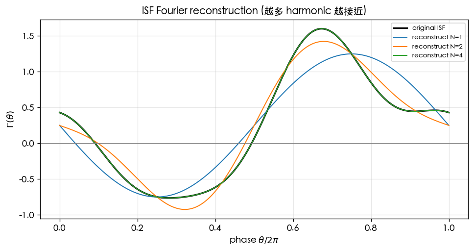
• Corresponding formula: [P1] Eq.(12) (partial sum $\Gamma_N=\frac{c_0}{2}+\sum_{n=1}^{N}c_n\cos(n\omega_0\tau+\theta_n)$).
• How to read it: $N=1$ captures only the fundamental and has the largest error; by $N=4$ the curves almost coincide. In practice the ISF's energy concentrates in the low-order harmonics, so a handful of terms is enough to compute phase noise accurately.
• Toy-model note: this ISF is a synthetic teaching waveform, not a transistor-level extraction.
• Full script: simulations/lab_05_fourier_isf.py.

Figure 2: the coefficient spectrum $c_n$ (with Parseval verification)

The figure below (fig_coefficients from lab_05, n_harmonics=8) plots $c_n$ as a bar chart (the coefficient spectrum) and marks the Parseval check $\sum_{n=0}^{\infty}c_n^2=2\Gamma_{rms}^2$ ([P1] Eq.(20), derived in detail on the next page).

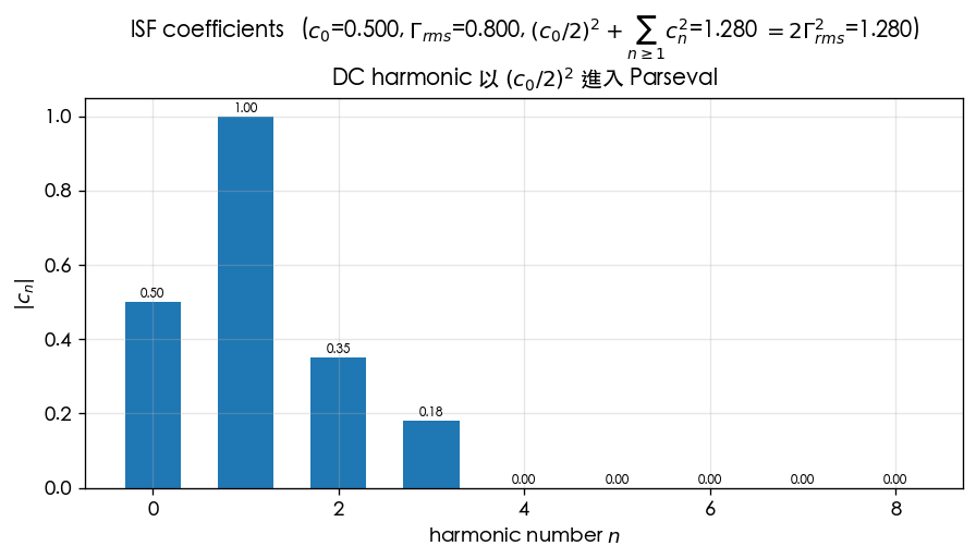
• Corresponding formulas: the $c_n$ of [P1] Eq.(12); the $\sum c_n^2=2\Gamma_{rms}^2$ of [P1] Eq.(20).
• How to read it: each bar's height is that harmonic's "weight" in the phase noise. The $c_0$ bar is critical — as soon as it is nonzero, close-in $1/f^3$ appears. The low-order bars dominate; the high orders decay quickly.
• The detailed Parseval derivation and $\Gamma_{rms}$ are in rms_isf.

Figure 3: $c_0$ for symmetric vs. asymmetric waveforms

The figure below (fig_symmetric_vs_asymmetric from lab_05) contrasts two toy ISFs: the symmetric $\Gamma=\cos\theta$ ($c_0=0$) and the asymmetric $\Gamma=\cos\theta+0.4$ ($c_0=0.8$), highlighting that only $c_0\neq0$ upconverts $1/f$ noise.

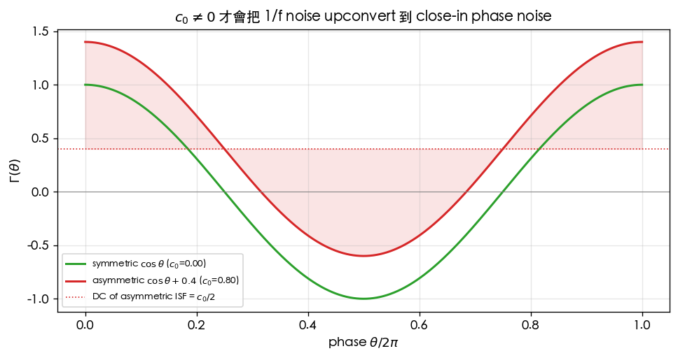
• Corresponding formulas: $c_0$ ([P1] Eq.(12)); its consequence, the $1/f^3$ corner of [P1] Eq.(24).
• How to read it: on the left, the symmetric waveform has zero mean and the DC bar disappears → no $1/f^3$; on the right, the whole curve is lifted and the DC bar pops out → close-in noise degrades. In design terms, "making the waveform symmetric" means "flattening this DC bar".
• Toy-model note: gamma_symmetric/gamma_asymmetric are pedagogical toy ISFs, not transistor-level (see the isf_utils.py docstring).
• Design-side extension: symmetry.

Numerical example (building a feel for the numbers)

Take the ideal-LC $\Gamma(\theta)=-\sin\theta$ and hand-compute the first few coefficients.

View $-\sin x$ as a Fourier expansion of itself: $-\sin x=c_1\cos(x+\theta_1)$, where $\cos(x+\theta_1)=\cos x\cos\theta_1-\sin x\sin\theta_1$; for this to equal $-\sin x$ requires $\theta_1=\pi/2$ (then $\cos(x+\pi/2)=-\sin x$), hence $c_1=1$, $\theta_1=\pi/2$.

• $c_0=\dfrac{1}{\pi}\displaystyle\int_0^{2\pi}(-\sin x)\,dx=0$ (odd function, zero DC).
• $c_1=1$, $c_n=0$ ($n\ge2$).
• Feel: the ideal-LC ISF is a "clean single fundamental" — all the energy sits in $c_1$. So it folds noise back mainly from near $\omega_0$ ($1/f^2$), and since $c_0=0$ there is, ideally, no $1/f^3$. The next page shows $\sum c_n^2=c_1^2=1=2\Gamma_{rms}^2$ ⟹ $\Gamma_{rms}=1/\sqrt{2}\approx0.707$.

Worked examples

Two problems in the strict format: problem → step-by-step substitution (with units) → result → dimension check → one-line Python verification. Problem 1 hand-computes $c_0,c_1,c_2$ and cross-checks with compute_fourier_coefficients; Problem 2 computes one harmonic's contribution to the phase noise.

Example 1 (hand-compute the first few $c_n$, then cross-check in code): given the toy ISF $\Gamma(\theta)=0.25-\sin\theta+0.35\sin2\theta+0.18\cos3\theta$ (the synthetic waveform used in the lab_05 reconstruction figure), hand-compute $c_0,c_1,c_2,c_3$.

Step by step (read the coefficients off directly; no integration needed): compare $\Gamma$ term by term with the standard expansion $\Gamma=\dfrac{a_0}{2}+\sum_n[a_n\cos n\theta+b_n\sin n\theta]$:

1. DC: the constant term of $\Gamma$ is $0.25$, i.e. the mean $=0.25$. Since the DC value $=a_0/2$, we get $a_0=0.5$, hence $c_0=a_0=0.5$.
2. Fundamental $n=1$: $\Gamma$ contains $-\sin\theta$ and no $\cos\theta$. Comparison gives $a_1=0$, $b_1=-1$. Hence $c_1=\sqrt{a_1^2+b_1^2}=\sqrt{0+1}=1$, $\theta_1=\operatorname{atan2}(-b_1,a_1)=\operatorname{atan2}(1,0)=\pi/2$.
3. Second harmonic $n=2$: contains $0.35\sin2\theta$ and no $\cos2\theta$. So $a_2=0$, $b_2=0.35$, hence $c_2=0.35$.
4. Third harmonic $n=3$: contains $0.18\cos3\theta$ and no $\sin3\theta$. So $a_3=0.18$, $b_3=0$, hence $c_3=0.18$.

Result: $c_0=0.5,\ c_1=1,\ c_2=0.35,\ c_3=0.18$ (the rest $\approx0$).

Dimension check: $\Gamma$ is dimensionless (notation); each $c_n$ is one of its Fourier amplitudes, likewise dimensionless; $\theta_n$ is rad (a phase) ✓.

Parseval cross-check (while we are at it): the strict relation (with the DC factor) is $\dfrac{c_0^2}{2}+\sum_{n\ge1}c_n^2=2\Gamma_{rms}^2$. Substituting: $\dfrac{0.5^2}{2}+(1^2+0.35^2+0.18^2)=0.125+1.1549=1.2799$, so $\Gamma_{rms}=\sqrt{1.2799/2}=0.800$. (Note: [P1] Eq.(20) writes $\sum_{n=0}^\infty c_n^2=2\Gamma_{rms}^2$ using the convention that the DC term carries no extra $1/2$; for a symmetric ISF with $c_0=0$ the two forms agree, but when $c_0\neq0$ remember the DC term's factor — see rms_isf.)

import numpy as np
from simulations.common.isf_utils import compute_fourier_coefficients, gamma_rms

theta = np.linspace(0.0, 2*np.pi, 4096, endpoint=True)
gamma = 0.25 - np.sin(theta) + 0.35*np.sin(2*theta) + 0.18*np.cos(3*theta)
a0, a, b, c, phase = compute_fourier_coefficients(theta, gamma, n_harmonics=4)
print("c0,c1,c2,c3 =", round(a0,3), round(c[1],3), round(c[2],3), round(c[3],3))
# -> c0,c1,c2,c3 = 0.5 1.0 0.35 0.18
print("Gamma_rms =", round(gamma_rms(theta, gamma),3))   # -> 0.8

Example 2 (one harmonic's contribution to phase noise): with the ISF of Example 1, a small tone of amplitude $I_0=1\ \mu\text{A}$ is injected at $2\omega_0+\Delta\omega$ (i.e. near the second harmonic). Take $q_{max}=1$ pC and $\Delta f=1$ MHz ($\Delta\omega=2\pi\times10^6$ rad/s). Find the phase-modulation amplitude and the relative single-sideband power this noise produces at offset $\Delta\omega$ from the carrier after downconversion via $c_2$.

Step-by-step substitution:

1. Only the $2$nd harmonic $c_2=0.35$ responds (the explicit algebra of Step 5: noise near $2\omega_0$ is moved to $\Delta\omega$ by $c_2$).
2. Phase-modulation amplitude (from Eq.(16/17) with $c_n\to c_2$):

$$\phi_p=\frac{I_0\,c_2}{2q_{max}\,\Delta\omega}=\frac{(10^{-6}\,\text{A})\times0.35}{2\times(10^{-12}\,\text{C})\times(6.283\times10^{6}\,\text{rad/s})}.$$

3. Denominator $=2\times10^{-12}\times6.283\times10^{6}=1.257\times10^{-5}\ \text{C}\cdot\text{rad/s}$; numerator $=3.5\times10^{-7}\ \text{A}$. Dividing gives $\phi_p=2.785\times10^{-2}\ \text{rad}$.
4. Relative single-sideband power ([P1] Eq.(18), $\left(\dfrac{I_0c_2}{4q_{max}\Delta\omega}\right)^2=(\phi_p/2)^2$):

$$P_{SBC}=\left(\frac{\phi_p}{2}\right)^2=\left(\frac{2.785\times10^{-2}}{2}\right)^2=1.939\times10^{-4}.$$

Result: $\phi_p\approx27.9$ mrad, $P_{SBC}\approx1.94\times10^{-4}=10\log_{10}\to-37.1$ dBc.

Dimension check: $\phi_p$: $\dfrac{\text{A}}{\text{C}\cdot(\text{rad/s})}=\dfrac{\text{A}}{(\text{A}\cdot\text{s})\cdot\text{s}^{-1}\cdot\text{rad}}=\dfrac{\text{A}}{\text{A}\cdot\text{rad}}=\text{rad}^{-1}$... in the simplification the rad of $\Delta\omega$ sits in the denominator, so $\phi_p$ carries rad ($C=\text{A}\cdot\text{s}$; the s of rad/s cancels the s of C) → rad ✓. $P_{SBC}=(\text{rad}/\text{rad})^2$ is dimensionless ✓ (a power ratio).

import numpy as np
I0, c2, qmax, dw = 1e-6, 0.35, 1e-12, 2*np.pi*1e6
phi_p = I0*c2/(2*qmax*dw)
P_sb  = (I0*c2/(4*qmax*dw))**2
print(round(phi_p*1e3,1), "mrad ;", round(10*np.log10(P_sb),1), "dBc")
# -> 27.9 mrad ; -37.1 dBc

• Feel: the same $1\ \mu\text{A}$ tone, if injected near the fundamental instead (using $c_1=1$ rather than $c_2=0.35$), makes $\phi_p$ larger by a factor of $1/0.35\approx2.86$ and the power larger by $(1/0.35)^2\approx8.2$ ($+9.1$ dB). This is the numerical face of "$c_n$ as mixer gains": the larger a harmonic's coefficient, the harder it folds that band's noise back.

(Full library: simulations/common/isf_utils.py.)

Applicability and failure conditions

Condition	When it holds	What happens when it fails
Oscillator in periodic steady state	$\Gamma$ is strictly $2\pi$-periodic, Fourier-expandable	during startup transients / under injection pulling, $\Gamma$ is not purely periodic
Noise is a small perturbation	linear superposition in Eq.(13) holds	large injection → harmonic interaction; the single-$c_n$ picture breaks down
Device noise is stationary	simple per-band bookkeeping	cyclostationary noise requires $\Gamma_{eff}=\Gamma\cdot\alpha$ (see effective_isf)
$\Gamma$ correctly extracted	coefficients are trustworthy	transient / adjoint simulation needed to obtain $\Gamma$

Key takeaways

• $\Gamma$ is a $2\pi$-periodic function, expandable as $\Gamma=\dfrac{c_0}{2}+\sum_{n\ge1}c_n\cos(n\omega_0\tau+\theta_n)$ ([P1] Eq.(12), p.183).
• The oscillator acts like a time-varying mixer: the $n$-th coefficient $c_n$ down-converts device noise near $n\omega_0$ to the carrier ([P1] Eq.(16), Fig. 8).
• $c_0$ (the DC coefficient; the DC value $=c_0/2$) upconverts baseband flicker noise into close-in $1/f^3$ ([P1] Eq.(15),(23),(24)).
• Waveform symmetry sets the parity of the coefficients: odd function ⟹ $c_0=0$ (no $1/f$ upconversion); half-wave symmetry ⟹ even harmonics vanish.
• Ideal LC: $c_0=0,\ c_1=1$, the rest zero; $\Gamma_{rms}=1/\sqrt2\approx0.707$.
• Numerically, compute_fourier_coefficients (trapezoidal rule; theta including both the $0$ and $2\pi$ endpoints) computes the coefficients.

Further reading

• Operational ISF definition (previous step): impulse_to_phase_shift
• Parseval and the rms ISF (next step): rms_isf
• How $c_n$ feeds $1/f^2$: white_noise_to_phase_noise
• How $c_0$ feeds $1/f^3$: flicker_noise_upconversion
• Design consequences of symmetry: symmetry
• Numerical-feel quick reference: numerical_feeling