Computing the ISF Directly from the Waveform — the Three Methods of [P1]'s Appendix

β: This English translation is in beta — the Traditional-Chinese original is the authoritative version.

Prerequisites: isf_definition (the definition of $\Gamma$ and the tangential-projection intuition), waveform_slope (the $1/\text{slope}$ heuristic and its divergence at waveform peaks) | Next: derivation_floquet_ppv (the rigorous adjoint/PPV — the source of this page's "ground truth"), lab_32 (the impulse method implemented on an equation-level ring)

The preceding pages define $\Gamma(\omega_0\tau)$ very carefully, but they leave one intensely practical question open: given an actual oscillator in hand (a SPICE netlist, a set of equations, or a measured steady-state waveform), how do you actually COMPUTE $\Gamma$? The appendix of [P1], "Calculation of the Impulse Sensitivity Function" ([P1] pp.192–193), gives three methods that form a spectrum from most accurate to fastest. This page transcribes all three verbatim, derives each step by step, and states each one's failure conditions clearly — then stages a three-way duel on a single van der Pol oscillator to turn "how far apart are they" into numbers.

Physical intuition (conclusion first): the three methods are really three tiers of the same thing. Method A (impulse injection) is "just run the experiment": poke the oscillator, measure the phase shift, assume nothing — so it is the most accurate and the slowest. Method B (closed form) replaces the experiment with geometry: it assumes that of the displacement you poke into the state, only the component tangent to the trajectory survives as phase — the experiment collapses into one inner product, computable from a single period of the waveform. Method C (first derivative) cuts once more: it assumes the denominator (the squared "speed" along the trajectory) is roughly constant, so $\Gamma$ becomes directly proportional to the waveform slope. Every cut buys speed and costs one more assumption that can fail. The core lesson of this page: Method B's tangential projection quietly assumes that "decaying amplitude perturbations leave no phase behind" — the moment amplitude-to-phase coupling (AM→PM) appears, it starts leaking.

Method A: direct measurement of the impulse response ([P1] Appendix A, p.192)

[P1]'s description on p.192 (transcribed): inject an impulse at different relative phases of the oscillation waveform and let the oscillator run for a few cycles; by sweeping the impulse injection time across one cycle and measuring the resulting time shift $\Delta t$, you obtain $h_\phi(t,\tau)$, using the conversion

$$\Delta\phi=2\pi\,\frac{\Delta t}{T},$$

where $T$ is the period of oscillation ([P1] p.192; this is exactly the phase–time conversion used in impulse_to_phase_shift). The paper adds that many SPICE implementations can perform the sweep automatically, and since each impulse needs only a few simulated cycles, it executes quickly; once $h_\phi(t,\tau)$ is found, "the ISF is calculated by multiplication with $q_{max}$" (compare [P1] Eq.(10): $h_\phi=\Gamma/q_{max}\cdot u(t-\tau)$, so $\Gamma=q_{max}h_\phi$ is the step height).

[P1]'s own verdict (p.192, verbatim): "This method is the most accurate of the three methods presented." — the most accurate of the three. The price is $N_{phase}$ transient runs (one per injection phase).

• Unit check: $\Delta\phi=2\pi\,[\text{s}]/[\text{s}]=$ rad ✓; $\Gamma=q_{max}\cdot h_\phi$, $[C]\cdot[\text{rad/C}]=$ dimensionless ✓.
• This site has implemented the method three times: a sinusoidal oscillator (lab_04, error ~0.001), a van der Pol (lab_15), and a MOS Level-1 equation-level ring (lab_32).
• Mind the wrap-around: fold $\Delta t$ back into $[-T/2,\,T/2)$ before converting, or you are off by a whole cycle (an implementation detail of lab_15/lab_32).

Method B: a closed form from the waveform ([P1] Appendix B, pp.192–193)

Step 1: project the perturbation onto the direction of motion — Eq. (31)

Consider the state-space trajectory of an $n$th-order system ([P1] Fig. 29, p.192: "State-space trajectory of an $n$th-order oscillator"). The effect of a group of external impulses is a perturbation vector $\Delta\vec X$ that instantly moves the state to $\vec X+\Delta\vec X$. The paper's key assumption sentence (p.192, verbatim): "As discussed earlier, amplitude variations eventually die away, but phase variations do not." To compute the equivalent time shift, project the perturbation onto the normalized velocity vector ([P1] Eq.(31), p.192):

$$l=\Delta\vec X\cdot\frac{\dot{\vec X}}{\bigl|\dot{\vec X}\bigr|}$$

• $l$ is the "equivalent displacement along the trajectory" (the paper's wording), and $\dot{\vec X}$ is the first derivative of the state vector (the trajectory's "velocity").
• Unit check: with all states as voltages, $[\Delta\vec X]=$ V and $\dot{\vec X}/|\dot{\vec X}|$ dimensionless → $l$ in V ✓ (a displacement carries the state's units).
• Hidden assumption #1: the inner product requires all state components to share one unit / one scale. If the state mixes V and A (e.g., an LC's $v_C,i_L$) you must normalize first — and the choice of normalization changes the answer (see "failure conditions").

The figure below replicates Fig. 29's state-space picture (left) and Fig. 30's three-method comparison (right — the Method C section refers back to it), computed on this site's van der Pol toy:

Conceptual replica, not a digitization of the originals. Left: corresponds to [P1] Fig. 29 (p.192), original caption verbatim: "State-space trajectory of an $n$th-order oscillator." — the original is an $n$-dimensional schematic hand drawing (no specific system); the replica instead actually computes a van der Pol (μ=2.0): thick line = limit cycle, thin line = the genuinely integrated re-converging trajectory after a kick $\Delta x=0.45$ on the $x$ axis (deliberately exaggerated for legibility), with $\Delta\phi$ marked as the same-time gap between the two trajectories and measured from late zero crossings as $-0.768$ rad ($-0.122$ cycles). Right: corresponds to [P1] Fig. 30 (p.193), original caption verbatim: "ISF's obtained from different methods.", original plot title "Calculation of Impulse Sensitivity Function" — the original's oscillator is not specified; the replica uses the same μ=0.2 vdP (the same machinery as the duel below), with the original's line styles: solid = 1st Method (A), dotted = 2nd Method (B), dashed = 3rd Method (C), and phase zero at the waveform minimum so the positive lobe precedes the negative one (the original's ordering). Honest difference: in the paper the 1st and 2nd methods nearly coincide and the dashed 3rd deviates (an $N$-identical-stage ring keeps Eq.(36)'s denominator constant); on this single-node vdP it is Methods B and C that nearly coincide (rms gap 0.134), while the impulse truth A departs near the waveform extrema (AM→PM, see the duel below). Numbers: $\Gamma_{rms}$ A/B/C $=0.7777$/$0.7097$/$0.6758$; rms $|B-A|=0.2365$, rms $|C-A|=0.3219$. Script: simulations/fig_p1_fig2930_replica.py (run with PYTHONPATH=. python simulations/fig_p1_fig2930_replica.py, about 1 s).

Step 2: displacement ÷ speed = time shift — Eq. (32)

A displacement $l$ along the trajectory is equivalent to a time shift of "$l$ divided by the speed $|\dot{\vec X}|$" ([P1] Eq.(32), p.193):

$$\Delta t=\frac{l}{\bigl|\dot{\vec X}\bigr|}=\Delta\vec X\cdot\frac{\dot{\vec X}}{\bigl|\dot{\vec X}\bigr|^{2}}$$

• Unit check: $[\text{V}]\cdot[\text{V/s}]/[\text{V/s}]^2=[\text{V}]/[\text{V/s}]=$ s ✓.
• Note the denominator becomes a square: one factor from normalizing the tangent vector, one from converting displacement to time. This is exactly the "divide by $\vert\partial\mathbf z/\partial\theta\vert^2$" step in the ideal-LC derivation of isf_definition.

Step 3: time shift → phase — Eq. (33)

([P1] Eq.(33), p.193):

$$\Delta\phi=2\pi\,\frac{\Delta t}{T}=\frac{2\pi}{T}\left(\Delta\vec X\cdot\frac{\dot{\vec X}}{\bigl|\dot{\vec X}\bigr|^{2}}\right).$$

Since $2\pi/T=\omega_0$, this is the "state-space projection" form often quoted: $\Delta\phi=\omega_0\,(\Delta\vec X\cdot\dot{\vec X})/|\dot{\vec X}|^2$.

Step 4: the special case of node-voltage states — Eq. (34)

If the state variables are node voltages and the impulse hits node $i$, the voltage jump is given by [P1] Eq.(9) ($\Delta V_i=\Delta q_i/C_i$), and Eq.(33) reduces to ([P1] Eq.(34), p.193):

$$\Delta\phi_i=\frac{2\pi}{T}\cdot\frac{\Delta q_i}{C_i}\cdot\frac{\dot v_i}{\bigl|\dot{\vec v}\bigr|^{2}}$$

where $\vert\dot{\vec v}\vert^2$ is the norm of the first derivative of the waveform vector and $\dot v_i$ is the derivative of the $i$-th node voltage (definitions verbatim from p.193).

• Step-by-step reading: $\Delta\vec X$ has only its $i$-th component nonzero ($=\Delta q_i/C_i$), so the inner product $\Delta\vec X\cdot\dot{\vec v}$ keeps only the $\dot v_i$ term.
• Unit check: $\dfrac{[\text{rad/s}]\cdot[\text{C}]/[\text{F}]\cdot[\text{V/s}]}{[\text{V/s}]^2}=\dfrac{[\text{rad/s}]\cdot[\text{V}]}{[\text{V/s}]}=$ rad ✓.

Step 5: rewrite with the normalized waveform — Eqs. (35), (36)

Substitute the normalized waveform $f$ of [P1] Eq.(1) ($v_i=V_{max}\,f_i(x)$, $x=\omega_0\tau$, with $f$'s derivatives taken with respect to $x$). Step by step:

$$\begin{aligned} \dot v_i&=\frac{d}{dt}\bigl[V_{max}f_i(x)\bigr]=V_{max}\,f_i'(x)\,\omega_0 &&(\text{chain rule},\ dx/dt=\omega_0)\\[4pt] \bigl|\dot{\vec v}\bigr|^{2}&=\sum_j\bigl(V_{max}f_j'\omega_0\bigr)^2=\omega_0^2V_{max}^2\,\bigl|\vec f\,'\bigr|^{2} &&(\text{equal amplitudes }V_{max}\text{: the identical-stage assumption})\\[4pt] \Delta\phi&=\omega_0\cdot\frac{\Delta q}{C_i}\cdot\frac{V_{max}f_i'\,\omega_0}{\omega_0^2V_{max}^2\bigl|\vec f\,'\bigr|^{2}} =\frac{\Delta q}{C_iV_{max}}\cdot\frac{f_i'}{\bigl|\vec f\,'\bigr|^{2}} &&(\text{every }\omega_0\text{ cancels}) \end{aligned}$$

Recognizing $C_iV_{max}=$ the node's maximum charge swing gives ([P1] Eq.(35), p.193, transcribed verbatim):

$$\Delta\phi=\frac{\Delta q}{q_i}\cdot\frac{f_i'}{\bigl|\vec f\,'\bigr|^{2}}$$

Notation note: [P1] Eq.(35) prints $q_i$ — the maximum charge swing of node $i$, i.e., the main text's (and this site's) $q_{max}$ for that node. $f_i'$ is "the derivative of the normalized waveform on node $i$" with respect to the phase $x$ (p.193, verbatim).

Comparing against the definition $\Delta\phi=\Gamma\,\Delta q/q_{max}$, the ISF reads off directly ([P1] Eq.(36), p.193):

$$\Gamma_i(x)=\frac{f_i'}{\bigl|\vec f\,'\bigr|^{2}}=\frac{f_i'}{\displaystyle\sum_{j=1}^{n}f_j'^{\,2}}$$

• Unit check: $f'$ is dimensionless (a dimensionless waveform differentiated with respect to rad) → $\Gamma$ dimensionless ✓.
• [P1]'s observation after Eq.(36) (p.193 — important; paraphrase plus the key sentence): this expression is maximum during transitions (where the derivative of $f$ is maximum), and that maximum value is inversely proportional to the maximum derivative — verbatim: "waveforms with larger slope show a smaller peak in the ISF function." This is the original source of the entire design intuition of waveform_slope.

Step 6: the second-order special case — Eq. (37), and the exact check on $f=\cos$

For a second-order system one can use the normalized waveform $f$ and its derivative $f'$ as the state variables, so the denominator of Eq.(36) keeps only two terms ([P1] Eq.(37), p.193):

$$\Gamma(x)=\frac{f'}{f'^{\,2}+f''^{\,2}}$$

where $f''$ is the second derivative of $f$ (defined on p.193). Verify the ideal sinusoid by hand ([P1]'s own sanity check on p.193 — here with the algebra written out): take $f(x)=\cos x$,

$$\begin{aligned} f'(x)&=-\sin x,\qquad f''(x)=-\cos x,\\[4pt] f'^{\,2}+f''^{\,2}&=\sin^2x+\cos^2x=1\qquad(\text{Pythagorean identity: the denominator is identically }1),\\[4pt] \Gamma(x)&=\frac{-\sin x}{1}=-\sin x. \end{aligned}$$

The paper's conclusion (p.193, verbatim): "In the case of an ideal sinusoidal oscillator $f=\cos(x)$, so that $\Gamma(\omega t)=-\sin(\omega t)$, which is consistent with the argument of Section III." Numerically we verify this to machine precision (simulations/fig_isf_three_methods.py prints max |Eq.(37) on cos - (-sin)| = 2.2e-16).

This step also resolves the "$1/\text{slope}$ diverges at the peak" paradox left open by waveform_slope:

• On transitions ($f'^2\gg f''^2$): $\Gamma\approx f'/f'^{\,2}=1/f'$ — precisely the regime where the $1/\text{slope}$ heuristic applies.
• Near peaks ($f'\to0$): the numerator $f'\to0$ while the denominator is held up by $f''^{\,2}$, so $\Gamma\approx f'/f''^{\,2}\to0$ — bounded, and tending to 0, no divergence.
• So $1/\text{slope}$ is the shadow of Eq.(37) in its slope-dominated limit; Eq.(37) is its rigorous parent formula, interpolating continuously between the two limits.
• But beware: Eq.(37) has its own sick point — if at some phase $f'$ and $f''$ approach 0 simultaneously (the waveform has a dead zone where both slope and curvature are flat), the denominator collapses and $\Gamma$ spikes (the waveform of worked example 2 below shows a spurious peak of $\vert\Gamma\vert\approx22.8$ at $x\approx2.81$). The higher-order form Eq.(36) is safer, its denominator being propped up by the other nodes' $f_j'^{\,2}$.

Method C: the first-derivative approximation — Eq. (38) ([P1] Appendix C, p.193)

The paper (p.193, paraphrase): this is a simplified version of the second approach. In certain cases the denominator of Eq.(36) shows little variation and can be approximated by a constant — the concrete example being a ring oscillator with $N$ identical stages (the stage transitions take turns, so $\sum_j f_j'^2$ is nearly constant). The denominator may then be approximated by $f_{max}'^{\,2}$ ([P1] Eq.(38), p.193):

$$\Gamma_i(x)=\frac{f_i'(x)}{f_{max}'^{\,2}}$$

The ISF is directly proportional to the waveform slope (divided by one constant). [P1]'s honest verdict (p.193, verbatim): "Although this method is approximate, it is the easiest to use and allows a designer to rapidly develop important insights into the behavior of an oscillator." [P1] Fig. 30 (p.193, "ISF's obtained from different methods") plots the three methods together; Method C (dashed) deviates in lobe height and detail but gets the shape right (see the right half of the replica figure in Method B, Step 1, for its conceptual replica).

• It is the engine of this site's interactive tool: interactive tool 7, the IsfSandbox (draw a waveform → see its ISF) uses precisely the [P2]-appendix variant of this slope approximation (each edge normalized by its own maximum slope, which is what lets rise/fall asymmetry produce $c_0\neq0$); this page is that widget's rigorous pedigree.
• The ring closed form of [P2] App. B (Eqs.(52)–(55), $\Gamma_{rms}=\sqrt{2\pi^2/(3\eta^3)}\,N^{-1.5}$, see rms_isf) is essentially the result of integrating Method C's triangular ISF.
• Failure: if the denominator $\sum_j f_j'^2$ varies strongly with phase (single-node view, few stages, badly distorted waveform), the constant-denominator approximation collapses — the μ=2 van der Pol in the duel below is exactly that case.

The three-method duel: one van der Pol, three answers — how far apart?

Theory done; now numbers. On a van der Pol oscillator ($\ddot x-\mu(1-x^2)\dot x+x=0$; the same toy as lab_15 and derivation_floquet_ppv), we kick charge into the $x$ axis ($x$ is this toy's "node voltage" — the vdP rewrites as a parallel RLC plus a nonlinear conductance with $x=v_C$, and a current impulse instantaneously changes exactly $x$), and put the three methods on stage:

• Method A (ground truth): impulse measurement at 24 phases (reusing lab_25's extract_isf_impulse_axis, machinery already cross-verified against the adjoint/PPV to rms 0.0023).
• Method B: Eq.(37) with $f=x/A$, $f'=y/(\omega_0A)$, $f''=\dot y/(\omega_0^2A)$, needing only one period of the waveform.
• Method C: Eq.(38), $f'/f_{max}'^{\,2}$.
• References: the harmonic limit $-\sin\theta$ (phase $\theta=0$ aligned to the waveform maximum, i.e., the $f\approx\cos\theta$ convention) and the rigorous adjoint/PPV curve (lab_25; the PPV is external literature, [E2] Demir 2000, not among the site's 5 PDFs).

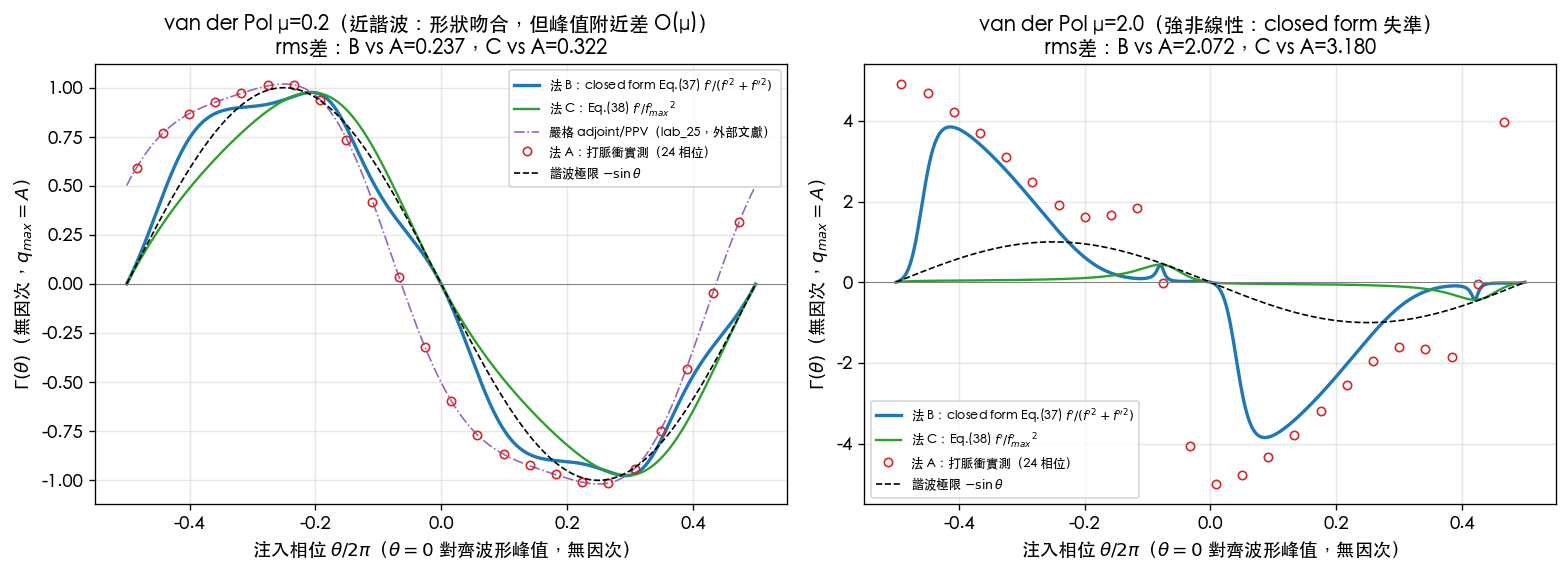
Parameter table: $\mu\in\{0.2,\,2.0\}$; impulse $\Delta q=0.02$ ($\Delta q/q_{max}\approx1\%$, $q_{max}\!=\!A\approx2$); 24 injection phases; RK4 step $2.5\times10^{-3}$ (impulse runs) / $T/6000$ (waveform grid); everything in normalized dimensionless units. Pedagogical toy model, not transistor-level. Full script: simulations/fig_isf_three_methods.py (run with PYTHONPATH=. python simulations/fig_isf_three_methods.py, about 3 s). Measured output:

--- mu = 0.2 ---
T  = 6.2989                          # -> 6.2989 (the 2π(1+μ²/16) prediction)
A  = 2.0004                          # -> 2.0004 (harmonic limit A=2)
Gamma_rms (Method B) = 0.7097        # -> 0.7097 (≈ the true-LC 1/√2=0.7071, not the representative 0.5)
Gamma_rms (Method A points) = 0.7777 # -> 0.7777 (the truth sits 9% above Method B)
peak |Gamma_B| = 0.9762              # -> 0.9762
peak |Gamma_A| = 1.0144              # -> 1.0144
rms |B - A(impulse)| = 0.2365        # -> 0.2365 (Method B's projection error)
rms |C - A(impulse)| = 0.3219        # -> 0.3219
rms |B - (-sin)|     = 0.078         # -> 0.078 (Method B essentially IS −sin)
rms |A - (-sin)|     = 0.28          # -> 0.28 (the truth left −sin long ago)
--- mu = 2.0 ---
Gamma_rms (Method B) = 1.9898        # -> 1.9898
Gamma_rms (Method A points) = 3.2151 # -> 3.2151 (Method B underestimates by 38%, ≈4.2 dB of phase noise)
peak |Gamma_A| = 5.0011              # -> 5.0011
rms |B - A(impulse)| = 2.072         # -> 2.072 (off the rails)
rms |C - A(impulse)| = 3.1803        # -> 3.1803 (collapse: one node, no N-stage sum to prop the denominator)
rms |B - A(impulse)| at mu=0.05 = 0.0586  # -> 0.0586 (shrink μ 4×, error shrinks 4.0×: error ∝ O(μ))
rms |B - PPV| (mu=0.2) = 0.237       # -> 0.237 (impulse ≡ PPV to 0.002, so the whole gap is Method B's projection error)

How to read the figure (and the numbers):

1. Left panel (μ=0.2, near-harmonic): Method B (blue) and Method C (green) are essentially $-\sin\theta$ (black dashed, rms gap 0.078), and $\Gamma_{rms}$ lands on the true-LC $1/\sqrt2$ (0.7097 vs 0.7071 — note this is the true-LC value $1/\sqrt2$, not the site's representative value 0.5). But the measured impulse points (red circles) and the rigorous PPV (purple dash-dot) coincide with each other and systematically leave Method B near the waveform peaks: at the peak, Method B says $\Gamma\approx-0.11$; the truth is $-0.59$.
2. That gap is not numerical noise — it is Method B's principled omission. Recall the assumption sentence of Step 1: "amplitude variations eventually die away, but phase variations do not" — it assumes that while an amplitude perturbation decays, it drags no phase along. The van der Pol's amplitude, however, back-modulates the instantaneous frequency (isochron twist, AM→PM): a radial offset $\Delta r$ decays as $e^{-\mu t}$, detunes the frequency by $O(\mu\Delta r)$ while decaying, and accumulates a phase $\int O(\mu\Delta r e^{-\mu t})dt=O(\Delta r)$ — the $\mu$ of the decay rate and the $\mu$ of the modulation strength cancel, leaving a finite residual phase. Only the oblique adjoint/PPV projection books this entry; the orthogonal tangential projection cannot (see derivation_floquet_ppv; this criterion is external literature, [E2]). Numerical evidence: dropping $\mu$ from 0.2 to 0.05 (4× smaller) shrinks the rms gap from 0.2365 → 0.0586 (exactly 4.0× smaller) — error $\propto O(\mu)$, concentrated exactly where Method B predicts $\Gamma\approx0$ (the peaks; precisely the "high AM–PM leaves residual phase even for peak injection" cell of the failure table in isf_definition).
3. Right panel (μ=2.0, strongly nonlinear): Method B's lobe height (3.85 vs the true 5.00), position, and width are all wrong, and $\Gamma_{rms}$ is underestimated by 38%; via $\mathcal L\propto\Gamma_{rms}^2$ ([P1] Eq.(21) — its $4\Delta\omega^2$ denominator is the SSB bookkeeping convention; the clean time-domain derivation gives $2\Delta\omega^2$, see white_noise_to_phase_noise) that is an underestimate of about 4.2 dB of phase noise. Method C (green) fares worse: the relaxation waveform's huge $f'_{max}$ squashes the whole ISF toward 0 (rms gap 3.18).
4. Engineering conclusion: for sign-off numbers use Method A (or the adjoint/PPV); use Method B for a "one-period quick look at the shape", quantitatively trustworthy on near-harmonic, low-AM–PM oscillators (error $\sim O(\mu)$); use Method C only in the "$N$ identical ring stages" scenario it was invented for (the dual-lobe ISF of lab_32 is the equation-level validation of that scenario).

Worked examples

Example 1: $\Gamma(\pi/6)$ via Eq.(37), connected to canonical Example A

Problem: ideal sinusoid $f(x)=\cos x$. Use the closed form Eq.(37) to find $\Gamma(\pi/6)$, then with $q_{max}=1$ pC, $\Delta q=1$ fC, $f_0=5$ GHz compute the phase step and timing error.

Step-by-step substitution (with units):

$$\begin{aligned} f'(\pi/6)&=-\sin\frac{\pi}{6}=-0.5,\qquad f''(\pi/6)=-\cos\frac{\pi}{6}=-0.8660,\\[4pt] f'^{\,2}+f''^{\,2}&=0.25+0.75=1\qquad(\text{the sinusoid's denominator is identically }1),\\[4pt] \Gamma(\pi/6)&=\frac{-0.5}{1}=-0.5\qquad(\text{dimensionless}),\\[4pt] \Delta\phi&=\frac{\vert\Gamma\vert\,\Delta q}{q_{max}}=\frac{0.5\times(1\times10^{-15}\,\text{C})}{1\times10^{-12}\,\text{C}}=5\times10^{-4}\ \text{rad},\\[4pt] \Delta t&=\frac{\Delta\phi}{2\pi f_0}=\frac{5\times10^{-4}\ \text{rad}}{2\pi\times5\times10^{9}\ \text{Hz}}=1.59\times10^{-14}\ \text{s}=15.9\ \text{fs}. \end{aligned}$$

• Result: the closed form gives $\Gamma=-0.5$ at $\theta=\pi/6$ — exactly the site's canonical Example A: $\vert\Gamma\vert=0.5$, $5\times10^{-4}$ rad, 15.9 fs.
• Dimension check: $\Gamma$ dimensionless ✓; $[\text{rad}]/[\text{rad/s}]=[\text{s}]$ ✓.
• Python verification:

import numpy as np
th = np.pi/6
fp, fpp = -np.sin(th), -np.cos(th)
g = fp/(fp**2 + fpp**2)
dphi = abs(g)*1e-15/1e-12
print(round(g, 4), round(dphi, 6), round(dphi/(2*np.pi*5e9)*1e15, 1))
# -> -0.5 0.0005 15.9  (Γ, Δφ [rad], Δt [fs])

Example 2: with second-harmonic distortion, by how much does Method C overshoot Method B?

Problem: a waveform with 30% second harmonic: $f(x)=\cos x+0.3\cos 2x$. Near the zero crossing, at $x=\pi/2$, compute $\Gamma$ with Method B (Eq.(37)) and Method C (Eq.(38)) and compare.

Step-by-step substitution: first the derivatives,

$$f'(x)=-\sin x-0.6\sin 2x,\qquad f''(x)=-\cos x-1.2\cos 2x.$$

At $x=\pi/2$: $\sin x=1$, $\sin 2x=0$, $\cos x=0$, $\cos 2x=-1$, so

$$\begin{aligned} f'&=-1,\qquad f''=+1.2,\\[4pt] \Gamma_B&=\frac{f'}{f'^{\,2}+f''^{\,2}}=\frac{-1}{1+1.44}=-0.4098,\\[4pt] f_{max}'^{\,2}&=1.9247\quad(\text{numerical extremum: }f'_{max}=1.3873\text{ at }x\approx58^\circ),\\[4pt] \Gamma_C&=\frac{f'}{f_{max}'^{\,2}}=\frac{-1}{1.9247}=-0.5196,\qquad \frac{\Gamma_C}{\Gamma_B}=1.27. \end{aligned}$$

• Result: with only 30% harmonic distortion, Method C already overshoots Method B by 27% at the ZC — because it forces "constant denominator" onto a waveform whose denominator does vary with phase. In $\Gamma^2$ terms that is roughly a 2 dB phase-noise error source.
• Bonus (Method B's own sick point): on this waveform, at $x\approx2.81$ both $f'$ and $f''$ pass near 0 simultaneously, and Eq.(37)'s $\vert\Gamma\vert$ spikes to 22.8 (a spurious peak) — Method B "cures the $1/\text{slope}$ divergence at the peak", but its own denominator can also die; scan $f'^{\,2}+f''^{\,2}$ for near-zeros before trusting it.
• Dimension check: dimensionless throughout ✓ ($f$, $f'$, $f''$, $\Gamma$ all dimensionless).
• Python verification:

import numpy as np
x = np.linspace(0, 2*np.pi, 200001)
fp  = -(np.sin(x) + 0.6*np.sin(2*x))
fpp = -(np.cos(x) + 1.2*np.cos(2*x))
i = np.argmin(np.abs(x - np.pi/2))
gB = fp[i]/(fp[i]**2 + fpp[i]**2)
gC = fp[i]/np.max(fp**2)
print(round(gB,4), round(gC,4), round(gC/gB,4), round(np.max(fp**2),4))
# -> -0.4098 -0.5196 1.2677 1.9247  (Γ_B, Γ_C, ratio, f'²max)

Applicability and failure conditions (all three methods)

Method	Needs	Cost	Accuracy	Failure conditions
A impulse (p.192)	re-runnable transients (simulator or equations)	$N_{phase}$ transients	most accurate of the three ([P1]'s words), cross-verified vs adjoint/PPV to rms ~0.002	$\Delta q$ too large (nonlinearity), unwrapped $\Delta t$, not yet in steady state
B closed form (Eqs.(31)–(37))	one period of the steady-state waveform + derivatives	one algebraic pass	error $\sim O(\mu)$ for near-harmonic, low-AM–PM oscillators; here rms 0.24 at μ=0.2	AM→PM (isochron twist): the orthogonal tangential projection misses the phase accumulated while the amplitude decays; mixed state units / scale choices change the answer; the denominator dies where $f'$ and $f''$ vanish together
C first derivative (Eq.(38))	one period of waveform slope	cheapest	qualitatively good inside "N identical ring stages" ([P1] Fig.30)	denominator $\sum_j f_j'^2$ varies strongly with phase: single node, few stages, strong distortion (here rms 3.18 at μ=2); rise/fall asymmetry needs per-edge normalization ([P2] App., the IsfSandbox's approach)

Key takeaways

• [P1]'s appendix gives three ways to compute the ISF: A impulse injection (most accurate) → B closed form $\Gamma=f'/(f'^{\,2}+f''^{\,2})$ (one period of waveform suffices) → C slope approximation $\Gamma=f'/f_{max}'^{\,2}$ (fastest, ring-specific) ([P1] Eqs.(31)–(38), pp.192–193).
• Method B's chain: project onto the unit tangent (Eq.(31)) → divide by speed to get time (Eq.(32)) → multiply by $2\pi/T$ to get phase (Eq.(33)) → node-voltage special case (Eq.(34)) → normalized waveform (Eqs.(35)(36)) → second-order special case (Eq.(37)).
• Substituting $f=\cos x$ into Eq.(37): the denominator $\sin^2+\cos^2=1$, so $\Gamma=-\sin x$ exactly — at the peak the numerator vanishes and the result stays bounded, resolving the $1/\text{slope}$ heuristic's divergence; $1/\text{slope}$ is just its limit where $f'^2\gg f''^2$.
• Method B's original sin is the orthogonal projection: it assumes "decaying amplitude leaves no phase". Turn on AM→PM (a van der Pol suffices) and the truth departs from Method B, with error $\propto O(\mu)$ concentrated at the peaks; under strong nonlinearity (μ=2) $\Gamma_{rms}$ is underestimated by 38% ≈ 4.2 dB of phase noise. The rigorous fix is the adjoint/PPV oblique projection (external literature).
• Method C is the engine of the IsfSandbox and of [P2]'s ring closed form; leave the "N identical stages" scenario and it collapses.
• Practical order: build intuition with C/B first; get sign-off numbers from A or the adjoint.

Further reading

• The definition of $\Gamma$ and the tangential-projection intuition: isf_definition
• The $1/\text{slope}$ heuristic (the shadow of this page's Eq.(37)): waveform_slope
• The rigorous adjoint/PPV (the full mathematics of Method B's missing term): derivation_floquet_ppv (external literature, [E2] Demir 2000)
• Three implementations of the impulse method: lab_04 (sinusoid), lab_15 (van der Pol), lab_32 (MOS Level-1 ring)
• The slope approximation, interactive: interactive tool 7, the IsfSandbox
• The ring $\Gamma_{rms}$ closed form (the integral of Method C): rms_isf