β: This English translation is in beta — the Traditional-Chinese original is the authoritative version.

Waveform slope and phase sensitivity

Prerequisites: impulse_to_phase_shift ($\Delta\phi=\Gamma\,\Delta q/q_{max}$ operational definition and $q_{max}=CV_{max}$), lti_vs_ltv (why the same impulse at different phases has different effect) | Next: symmetry, tank_swing

This page answers a very practical question, one you'll use during layout and bias design: at which phase of the waveform does the same lump of noise charge do the most damage? Intuitively you might guess "the peak — highest, most sensitive" — it's the opposite. ISF magnitude is, roughly, inversely proportional to waveform slope: where the slope is small (near the peak), $|\Gamma|$ is large and phase error is easiest to push; where the slope is large (at the ZC, zero crossing), noise is instead mostly converted into amplitude and pulled back.

Physical intuition (conclusion first): phase is "how fast the state point runs along the tangent of the limit cycle." At the peak, the state point moves "slowly, flatly" ($dV/dt\approx0$); nudge it sideways and it takes a long time along the time axis to return to where it would have been — equivalent to a large phase shift. At the ZC, the state point is "moving at full speed" ($dV/dt$ maximal); the same sideways nudge is quickly absorbed back onto the trajectory, leaving almost no phase (it mostly becomes a decaying amplitude perturbation). So "phases with small slope" are the danger zone.

Step 1: the inverse relation between ISF and slope

Return to the operational definition of impulse→phase ([P1] Eq.(10)–(11), p.182):

$$\Delta\phi=\frac{\Gamma(\omega_0\tau)}{q_{max}}\,\Delta q$$

A lump of charge $\Delta q$ produces a voltage jump $\Delta V=\Delta q/C$ ([P1] Eq.(9)). Translate this voltage jump into a "time-axis advance/delay": the waveform passes through this point with slope $\dot V=dV/dt$, and raising the voltage by $\Delta V$ is equivalent to shifting the waveform in time by

$$\Delta t\approx\frac{\Delta V}{\dot V}=\frac{\Delta q}{C\,\dot V}.$$

• Unit check: $[\text{V}]/[\text{V/s}]=[\text{s}]$ ✓.
• Converting to phase, $\Delta\phi=\omega_0\Delta t$:

$$\Delta\phi=\omega_0\frac{\Delta q}{C\,\dot V}\quad\Rightarrow\quad \Gamma\propto\frac{1}{\dot V}.$$

Step-by-step algebra: aligning this "shift approximation" with the ISF operational definition to see exactly what $\Gamma$ is proportional to. Set the $\Delta\phi$ from the above equation equal to the operational-definition expression $\Delta\phi=\Gamma\,\Delta q/q_{max}$:

$$\begin{aligned} \frac{\Gamma}{q_{max}}\,\Delta q&=\omega_0\,\frac{\Delta q}{C\,\dot V} \\[4pt] \Gamma&=\frac{q_{max}\,\omega_0}{C\,\dot V} \qquad(\text{cancel }\Delta q\text{ on both sides}) \\[4pt] \Gamma&=\frac{(C\,V_{max})\,\omega_0}{C\,\dot V}=\frac{\omega_0\,V_{max}}{\dot V} \qquad(\text{substitute }q_{max}=C\,V_{max}) \\[4pt] &=\frac{V_{max}}{\dot V/\omega_0}=\frac{V_{max}}{dV/d\theta}\qquad(\dot V=\omega_0\,dV/d\theta). \end{aligned}$$

• What each step uses: lines 1→2 are pure algebra (cancel $\Delta q$); lines 2→3 use $q_{max}=C V_{max}$ (the capacitance definition — $C$ cancels automatically, which is why ISF does not depend on node capacitance, only on waveform shape); lines 3→4 convert the time-domain slope to a phase-domain slope $\dot V=\omega_0\,dV/d\theta$ (chain rule).

• Meaning of the result: $\Gamma=V_{max}\big/(dV/d\theta)$ — ISF is proportional to $V_{max}$ and inversely proportional to the waveform's slope with respect to phase $dV/d\theta$.

• Check against a sinusoid: $V=V_{max}\cos\theta\Rightarrow dV/d\theta=-V_{max}\sin\theta$, so $\Gamma=V_{max}/(-V_{max}\sin\theta)=-1/\sin\theta$. This "$1/\sin$" is an artifact of the shift approximation and diverges where slope→0 (the peak); the rigorous LTV projection instead gives a bounded $\Gamma=-\sin\theta$ (with $\Gamma=0$ at the peak). Both say "small slope → dangerous," but they differ on whether it diverges — the shift approximation is only qualitatively valid where slope is nonzero; for quantitative work use $\Gamma=-\sin\theta$.

• Dimension check: $[\text{V}]/[\text{V}]=$ dimensionless ✓ ($\Gamma$ must be dimensionless); the intermediate expression $\dfrac{[\text{C}]\cdot[\text{rad/s}]}{[\text{F}]\cdot[\text{V/s}]}=\dfrac{[\text{C}][\text{s}^{-1}]}{[\text{C/V}][\text{V/s}]} =\dfrac{[\text{C}][\text{s}^{-1}]}{[\text{C}][\text{s}^{-1}]}=$ dimensionless ✓ (rad does not count as a dimension).

• Conclusion: ISF magnitude is inversely proportional to instantaneous slope $\dot V$. Large slope → small $|\Gamma|$ (insensitive); small slope → large $|\Gamma|$ (sensitive).

• For an ideal sinusoid $V=\cos\theta$, $\dot V\propto-\sin\theta$, so the "shift" approximation $\Gamma(\theta)\propto1/\sin\theta$ only holds where slope is nonzero; the rigorous LC ISF is $\Gamma(\theta)=-\sin\theta$ ($\Gamma=0$ at the peak $\theta=0$, $|\Gamma|$ maximal at the ZC $\theta=\pi/2$).

The divergence problem now has its rigorous resolution (resolved): the $1/\text{slope}$ divergence at the peak has an official "parent formula" — the closed form of [P1]'s appendix (Eq.(37), p.193) $\Gamma=f'/(f'^{\,2}+f''^{\,2})$: on transitions ($f'^{\,2}\gg f''^{\,2}$) it degenerates into this page's $1/f'$ heuristic; near the peak the numerator $f'\to0$ while the denominator is held up by $f''^{\,2}$, so $\Gamma\to0$ — bounded, no divergence. Substituting $f=\cos$ gives the denominator $\sin^2+\cos^2=1$ and $\Gamma=-\sin$ exactly. For the full derivation, the verbatim transcription of [P1]'s three ISF calculation methods, and the numerical duel, see isf_from_waveform.

A common direction confusion needs to be spelled out here: the "shift" picture above, "$\Delta t=\Delta V/\dot V$," describes "how much the threshold-crossing time moves after the waveform is perturbed by voltage" — that is threshold-crossing sensitivity, where a large slope makes timing more stable (this is another angle on "fast transitions help"). By contrast, $\Gamma=-\sin\theta$ describes excess-phase sensitivity: zero at the peak, maximal at the ZC. The two appear contradictory but are actually different questions: threshold crossing asks "when does the edge cross the threshold"; excess phase asks "how much is the limit cycle pushed tangentially." This page, and the design rules across the whole site, follow [P1]'s ISF $\Gamma$ (excess phase): $|\Gamma|$ is maximal at the ZC (the high-slope crossing point) and minimal at the peak. This is exactly what the figure below shows.

Step 2: reading the LC waveform vs. ISF overlay

The figure below overlays the ideal LC waveform $V(\theta)=\cos\theta$ with its ISF $\Gamma(\theta)=-\sin\theta$:

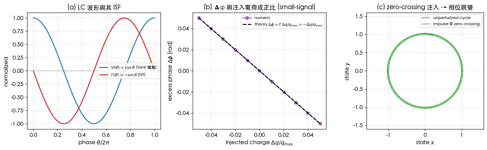
How to read this figure:

• Peak/trough ($\theta=0,\pi$, $V$ at an extremum, $dV/d\theta=0$): $\Gamma=0$. Injecting charge here → pure amplitude perturbation → pulled back by amplitude restoration → leaves almost no phase. This is the "safe" phase.
• Zero crossing, ZC ($\theta=\pi/2,3\pi/2$, $V=0$, slope maximal): $|\Gamma|$ is maximal. Injecting charge here → pure phase jump → persists permanently. This is the "dangerous" phase.
• Compare to [P1] Fig. 4: the same impulse applied at the peak versus at the ZC produces completely different tangential/radial decomposition in state space — this is the signature of the oscillator being an LTV (linear time-varying) system (claim C1).

This is a pedagogical toy model (not transistor-level): an idealized LC in the sinusoidal steady state. A real LC, with tank loss and a nonlinear transconductor, will not give a perfect $-\sin$ ISF, but the qualitative conclusion "peak safe, ZC dangerous" holds. Full script: simulations/lab_02_lc_toy_model.py.

Step 3: why "fast transitions" help ring oscillators

A ring oscillator's waveform is not sinusoidal but closer to a square wave — spending most of its time "pinned at the rail" and rushing through the ZC only during the switching instant (the transition). Its ISF is therefore concentrated near the transition ([P2] Fig. 6, p.793; Fig. 5 shows the peak/lobe narrowing with $N$):

• On the rail (flat top): $\dot V\approx0$ should in theory be very sensitive — but the device is usually not conducting / not injecting noise at that moment ($\alpha\approx0$, see device_noise_mapping), so the effective ISF stays small.
• During the transition: $\dot V$ is maximal → the bare $\Gamma$ is small; but the device is switching at full tilt, and noise is maximal ($\alpha$ large).
• Multiplying the two together: the ring's effective ISF $\Gamma_{eff}=\Gamma\cdot\alpha$ has its energy concentrated at the transition.

Why a fast transition (steep edge) helps, for two mutually reinforcing reasons:

1. Shortens the danger window: the faster the transition, the narrower the time window in which the device is "fully on, crossing the edge," so less noise is collected into phase during this "exposure time" → $\Gamma_{rms}$ drops (the ring's $\Gamma_{rms}\propto N^{-3/2}$ trend is also tied to each stage's transition getting steeper; see lc_vs_ring).
2. Improves threshold-crossing immunity: the steeper the edge, the smaller $\Delta t=\Delta V/\dot V$ — the same voltage noise produces less timing jitter. This is the same principle behind "fast slew rate → low jitter" on a SerDes data path (see serdes_clocking_connection).

Numerical example (building intuition)

Using canonical numbers to estimate "the phase difference from the same $\Delta q$ at peak vs. ZC."

Take $q_{max}=1$ pC, $\Delta q=1$ fC, $f_0=5$ GHz. Ideal LC $\Gamma(\theta)=-\sin\theta$:

• At the ZC ($\theta=\pi/2$, $\Gamma=-1$, maximum sensitivity):

$$\Delta\phi=\frac{|\Gamma|\,\Delta q}{q_{max}}=\frac{1\times10^{-15}}{10^{-12}}=10^{-3}\ \text{rad}\;\Rightarrow\;\Delta t=\frac{10^{-3}}{2\pi\cdot5\times10^9}=31.8\ \text{fs}.$$

• At the peak ($\theta=0$, $\Gamma=0$): $\Delta\phi=0$ rad, $\Delta t=0$ (ideal; real devices show residual leakage).
• At an intermediate phase ($\theta=\pi/6$, $\Gamma=-0.5$, i.e., canonical example A's $\Gamma=0.5$):

$$\Delta\phi=\frac{0.5\times10^{-15}}{10^{-12}}=5\times10^{-4}\ \text{rad}\;\Rightarrow\;\Delta t=15.9\ \text{fs}.$$

• Intuition: the same 1 fC produces ~32 fs at the ZC but ~0 fs at the peak. Position (phase) matters more than magnitude — this is why, during layout, you should avoid coupling large noise sources (e.g., a switching tail current source, supply ripple) into "low-slope" phase windows.

Turning slope into design knobs (checklist)

Knob	How	Mechanism	Cost / notes
Increase transition slew rate	Larger delay-cell drive, lower load capacitance	Shortens the danger window, lowers $\Gamma_{rms}$, lowers threshold jitter	More current → higher power
Move large noise sources away from sensitive phases	Time tail-current switching, charge injection to align with the peak/low-$\alpha$ window	Inject where $\vert \Gamma_{eff}\vert$ is small	Requires timing planning
Increase swing (raise $\dot V$)	Large tank swing (LC), full-rail (ring)	High slope → low threshold sensitivity, and raises $q_{max}$ at the same time	Limited by headroom (see tank_swing)
Avoid the device still conducting during the "flat-top" period	Make the device conduct only at low-$\Gamma$ phase	Offsets cyclostationary $\alpha$ from $\Gamma$	Requires effective-ISF analysis

Validity and failure conditions

Condition	When it holds	When it fails
Small perturbation, linear projection	$\Gamma\propto1/\dot V$ approximation valid	Strong nonlinearity or large injection changes the ISF itself
Nonzero slope	$\Delta t=\Delta V/\dot V$ is defined	At the exact peak ($\dot V=0$), take the limit $\Gamma=0$ (pure amplitude)
Amplitude perturbation decays	Phase alone can be tracked	With strong AM–PM, even peak injection can leave residual phase

Worked examples

The following two problems work out "the same $\Delta q$, injected at high vs. low slope, how different is $\Delta\phi$" with concrete $\Gamma$ values, continuing with the canonical $q_{max}=1$ pC, $\Delta q=1$ fC, $f_0=5$ GHz, ideal LC $\Gamma(\theta)=-\sin\theta$.

Example 1 (high-slope vs. low-slope, ratio of $\Delta\phi$ for the same $\Delta q$) Inject the same lump $\Delta q=1$ fC at the ZC ($\theta=\pi/2$, slope maximal, $|\Gamma|=1$) and "near the peak" ($\theta=\pi/6=30^\circ$, slope small, $|\Gamma|=\sin(\pi/6)=0.5$). Find $\Delta\phi$ at each point and their ratio.

Step-by-step substitution (with units), using $\Delta\phi=\dfrac{|\Gamma|\,\Delta q}{q_{max}}$:

$$\begin{aligned} \Delta\phi_{ZC}&=\frac{|{-}\sin(\pi/2)|\cdot\Delta q}{q_{max}}=\frac{1\times(1\times10^{-15}\,\text{C})}{1\times10^{-12}\,\text{C}}=1\times10^{-3}\ \text{rad}, \\[4pt] \Delta\phi_{30^\circ}&=\frac{|{-}\sin(\pi/6)|\cdot\Delta q}{q_{max}}=\frac{0.5\times10^{-15}}{10^{-12}}=5\times10^{-4}\ \text{rad}, \\[4pt] \frac{\Delta\phi_{ZC}}{\Delta\phi_{30^\circ}}&=\frac{|\Gamma(\pi/2)|}{|\Gamma(\pi/6)|}=\frac{1}{0.5}=2. \end{aligned}$$

• Result: the phase shift at the high-slope point (ZC) is 2× the low-slope point ($30^\circ$) — because the $\Gamma$ values differ by exactly 2×. Note the ZC is the phase where $|\Gamma|$ is maximal, i.e., most dangerous.
• Dimension check: $\dfrac{[\text{dimensionless}]\cdot[\text{C}]}{[\text{C}]}=[\text{rad}]$ (dimensionless) ✓; the ratio is dimensionless ✓.
• One-line Python check:

import numpy as np
from simulations.common.isf_utils import gamma_lc_ideal, impulse_to_phase_step
g_zc = abs(gamma_lc_ideal(np.pi/2));  g_30 = abs(gamma_lc_ideal(np.pi/6))
d_zc = impulse_to_phase_step(1e-15, g_zc, 1e-12)
d_30 = impulse_to_phase_step(1e-15, g_30, 1e-12)
print(d_zc, d_30, d_zc/d_30)   # -> 0.001  0.0005  2.0

Example 2 (near-immunity at the peak + converting to timing error for intuition) The same lump $\Delta q=1$ fC is injected at the "positive peak" ($\theta=0$, slope $=0$, $\Gamma=0$). Find $\Delta\phi$ and $\Delta t$; then compare against Example 1's ZC injection, converted to a timing error at $f_0=5$ GHz.

Step-by-step substitution (with units):

$$\begin{aligned} \Delta\phi_{peak}&=\frac{|{-}\sin 0|\cdot\Delta q}{q_{max}}=\frac{0\times10^{-15}}{10^{-12}}=0\ \text{rad}\;\Rightarrow\;\Delta t_{peak}=0\ \text{s}, \\[4pt] \Delta t_{ZC}&=\frac{\Delta\phi_{ZC}}{2\pi f_0}=\frac{1\times10^{-3}\ \text{rad}}{2\pi\times5\times10^{9}\ \text{Hz}} =\frac{10^{-3}}{3.1416\times10^{10}}\ \text{s}\approx3.18\times10^{-14}\ \text{s}=31.8\ \text{fs}. \end{aligned}$$

• Result: ideal peak injection → $\Delta\phi=0$, $\Delta t=0$ (pure amplitude perturbation, pulled back by amplitude restoration); the same charge injected at the ZC → 31.8 fs. Position (phase) matters more than magnitude: the difference isn't a few percent — it's 0 versus 32 fs.
• Dimension check: $[\text{rad}]/[\text{rad/s}]=[\text{s}]$ ✓ ($2\pi f_0$ is in rad/s).
• One-line Python check:

import numpy as np
from simulations.common.isf_utils import gamma_lc_ideal, impulse_to_phase_step
from simulations.common.noise_utils import phase_to_time_error
for th in (0.0, np.pi/2):
    dphi = impulse_to_phase_step(1e-15, abs(gamma_lc_ideal(th)), 1e-12)
    print(f"theta={th:.3f}: dphi={dphi:.1e} rad, dt={phase_to_time_error(dphi,5e9)*1e15:.1f} fs")
# theta=0.000: dphi=0.0e+00 rad, dt=0.0 fs ; theta=1.571: dphi=1.0e-03 rad, dt=31.8 fs

Both problems are pedagogical toys (ideal LC $-\sin$, not transistor-level): a real waveform has residual AM–PM at the peak, so $\Delta t$ will not be strictly 0.

Key takeaways

• ISF magnitude is, roughly, inversely proportional to waveform slope: small slope (peak) → large $|\Gamma|$, dangerous; large slope (ZC) → small $|\Gamma|$, safe.
• Ideal LC: $\Gamma=-\sin\theta$, $\Gamma=0$ at the peak, $|\Gamma|$ maximal at the ZC (see figure).
• Fast transitions give a double benefit: shortening the "danger window" lowers $\Gamma_{rms}$, and improving threshold-crossing immunity lowers timing jitter.
• Same 1 fC lump: ~32 fs when injected at the ZC, ~0 fs at the peak (5 GHz, $q_{max}=1$ pC) — position matters more than magnitude.
• A ring's effective ISF concentrates at the transition; keep large noise sources away from phases where $|\Gamma_{eff}|$ is large.

Further reading

• Full impulse→phase derivation: impulse_to_phase_shift
• The rigorous parent formula of $1/\text{slope}$ and [P1]'s three ISF calculation methods: isf_from_waveform
• LTV (why the same impulse has a different effect at different phases): lti_vs_ltv
• Symmetry and $c_0$: symmetry
• Swing and $q_{max}$: tank_swing
• Cyclostationary $\alpha$: device_noise_mapping