β: This English translation is in beta — the Traditional-Chinese original is the authoritative version.

The Theoretical Ceiling of FOM

Prerequisites: tank_swing (FOM definition and the phase-noise × power trade-off), white_noise_to_phase_noise ([P1] Eq.(21) and the factor-of-2 convention), lc_vs_ring ([P2] Eq.(23) ring FOM, the $-91$ dBc/Hz example) | Next: real_oscillator_topologies, pll_noise_budget

This page answers three questions every VCO designer eventually asks:

1. Does FOM (figure of merit — the oscillator quality metric) have a physical upper bound? What is it, and what sets it?
2. The best published LC designs sit around FOM $\approx190$ dB — how many dB below the ceiling are they?
3. Why does the ring oscillator inherently trail LC by about 25 dB? Which term eats each dB of that gap?

Physical intuition (conclusion first): FOM is constructed to exactly cancel $(f_0/\Delta f)^2$ and power $P$. What's left are only two things: nature's price list, $kT$ (thermal-noise energy in a 1 Hz bandwidth vs. 1 mW), which comes to 173.8 dB at 300 K; and the topology noise factor $F_{eff}$ — how much your circuit amplifies $kT$ (ring: $F_{eff}\ge3.6$, ceiling 168.3 dB) or beats it down with high-$Q$ energy storage (LC: $F_{eff}\propto 1/Q^2$, ceiling rises 20 dB per decade of $Q$). So there is no single magic number: the ceiling is a "family," and which member you land on is set by what physics you allow into $F_{eff}$.

Step 0: FOM's definition and sign convention

This page uses the positive-value convention (bigger is better, the most common form in survey tables):

$$\mathrm{FOM}\;=\;-\mathcal{L}(\Delta f)\;+\;20\log_{10}\!\left(\frac{f_0}{\Delta f}\right)\;-\;10\log_{10}\!\left(\frac{P}{1\ \text{mW}}\right)\qquad[\text{dB}]$$

• $\mathcal{L}(\Delta f)$: SSB phase noise at offset $\Delta f$, in dBc/Hz (negative, so $-\mathcal{L}$ is positive).
• $f_0$: carrier frequency [Hz]; $\Delta f$: offset frequency [Hz]; $P$: total DC power dissipation [W], normalized to 1 mW.
• Comparison with tank_swing: that page writes $\mathrm{FOM}'=\mathcal{L}-20\log_{10}(f_0/\Delta f)+10\log_{10}(P/1\text{mW})$ — the same quantity with the sign flipped ($\mathrm{FOM}=-\mathrm{FOM}'$; under that convention more negative is better). Both forms appear in the literature; this page uses the positive convention, so numerically the ring example's $\mathrm{FOM}=165.0$ dB here is that page's $\mathrm{FOM}'=-165.0$ dB.
• A hidden reference unit: the "per Hz" in $\mathcal{L}$ is really "sideband power in a 1 Hz measurement bandwidth ÷ carrier power." Writing out this $B_{ref}=1$ Hz explicitly is what makes FOM's log argument strictly dimensionless; FOM's full reference basis is "1 Hz bandwidth, 1 mW power." The next step shows this isn't pedantry — it's exactly what lets $kT$ appear cleanly.
• Dimension check: all three terms are $10\log_{10}$ of dimensionless ratios ($\mathcal{L}_{lin}B_{ref}$, $(f_0/\Delta f)^2$, $P/P_{ref}$) → dB ✓.

Step 1: the reference constant — 173.8 dB is $1\cdot kT$, not $2kT$

Suppose some topology's phase noise in the $1/f^2$ (white-noise) region can be arranged into the following universal form (the next two steps show both ring and LC reduce to this):

$$\mathcal{L}_{lin}(\Delta f)\;=\;F_{eff}\cdot\frac{kT}{P}\cdot\left(\frac{f_0}{\Delta f}\right)^2\qquad\left[\tfrac{1}{\text{Hz}}\right]$$

where $F_{eff}$ is the dimensionless topology noise factor (this equation is its definition). Unit check: $\dfrac{kT}{P}=\dfrac{[\text{J}]}{[\text{W}]}=[\text{s}]=\dfrac{1}{[\text{Hz}]}$, multiplied by the dimensionless $F_{eff}(f_0/\Delta f)^2$ this gives exactly the per-Hz units $\mathcal{L}_{lin}$ needs ✓. Substitute into the FOM definition and cancel step by step:

$$\begin{aligned} \mathrm{FOM} &=-10\log_{10}\!\left(F_{eff}\,\frac{kT\,B_{ref}}{P}\Big(\frac{f_0}{\Delta f}\Big)^{2}\right) +10\log_{10}\!\left(\Big(\frac{f_0}{\Delta f}\Big)^{2}\right) -10\log_{10}\!\left(\frac{P}{P_{ref}}\right)\\[4pt] &=-10\log_{10}\!\left(F_{eff}\cdot\frac{kT\,B_{ref}}{P}\cdot\frac{P}{P_{ref}}\right) \qquad\text{(the two }(f_0/\Delta f)^{2}\text{ terms cancel)}\\[4pt] &=\underbrace{-10\log_{10}\!\left(\frac{kT\,B_{ref}}{P_{ref}}\right)}_{\equiv\,C_{ref}(T)\text{, temperature-only}}\;-\;10\log_{10}F_{eff}. \end{aligned}$$

• What each step uses: going from line 1→2, $(f_0/\Delta f)^2$ cancels exactly between $-\mathcal{L}$ and $+20\log_{10}(f_0/\Delta f)$; going from line 2→3, $P$ cancels exactly between $kT/P$ and $P/P_{ref}$. These two cancellations are precisely the reason FOM was invented (to normalize away the "$\mathcal{L}\times P\approx$ constant" trade-off — see tank_swing step 4).
• Dimension check: $\dfrac{kT\,B_{ref}}{P_{ref}}=\dfrac{[\text{J}][\text{Hz}]}{[\text{W}]}=\dfrac{[\text{W}]}{[\text{W}]}$, dimensionless ✓ — the $B_{ref}=1$ Hz hidden in step 0 is exactly what completes $kT$'s dimensions here.
• Physical meaning: $kT\cdot(1\ \text{Hz})$ is the available thermal-noise power a resistor can deliver in a 1 Hz bandwidth ($kT\approx4.14\times10^{-21}$ J @ 300 K); $C_{ref}$ is simply "how many dB is 1 mW above the thermal-noise floor."

Numerically ($k=1.380649\times10^{-23}$ J/K, $T=300$ K): $kT=4.142\times10^{-21}$ J, $kT\cdot1\,\text{Hz}/1\,\text{mW}=4.142\times10^{-18}$, $C_{ref}=-10\log_{10}(4.142\times10^{-18})=173.83$ dB.

$$\boxed{\;\mathrm{FOM}\;=\;173.8\ \text{dB}\;-\;10\log_{10}F_{eff}\qquad(T=300\ \text{K})\;}$$

⚠️ A memorization trap (worked out on this site — don't get it wrong): quick notes often write this constant as "$-10\log_{10}(2kT/1\text{mW})=173.8$" — wrong. $2kT$ pairs with $170.8$ dB; $173.8$ dB pairs with $1\cdot kT$. This page's derivation naturally lands on $1\cdot kT$: because [P2] Eq.(23) is printed in exactly the $kT/P$ form (step 2), while the LC reduction (step 3) folds all factors of 2 and 4 into $F_{eff}$. Every factor-of-2 convention (SSB's /4 vs. the time-domain /2) lives inside $F_{eff}$ and only shifts FOM by 3.01 dB total; $C_{ref}$ itself is convention-free.

import numpy as np
kB, T = 1.380649e-23, 300.0
print(round(-10*np.log10(kB*T*1.0/1e-3), 2))   # -> 173.83
print(round(-10*np.log10(2*kB*T/1e-3), 2))     # -> 170.82 (the 2kT pairing, often misremembered as 173.8)
print(round(10*np.log10(kB*290.0/1e-3), 2))    # -> -173.98 (the RF world's famous -174 dBm/Hz thermal-noise floor)

• Bonus: converting $kT$ using $T_0=290$ K (the IEEE noise-figure reference temperature, from Friis 1944, external literature, not among the five source PDFs, full citation at page bottom) to dBm/Hz gives the famous $-174$ dBm/Hz; 300 K gives $-173.83$, both round to $-174$.
• Temperature effect: $C_{ref}$ drops about $0.14$ dB per 10 K rise ($C_{ref}(310\,\text{K})-C_{ref}(300\,\text{K})=-0.142$ dB) — remember this slope when comparing FOM measured at different temperatures.

Step 2: ring — one reduction of [P2] Eq.(23), ceiling 168.3 dB

[P2] Eq.(23), p.796 (verified against the original PDF, leading coefficient $8/(3\eta)$) is already in universal form:

$$\mathcal{L}_{lin}\{\Delta f\}=\frac{8}{3\eta}\cdot\frac{kT}{P}\cdot\frac{V_{DD}}{V_{char}}\cdot\left(\frac{f_0}{\Delta f}\right)^{2} \;\;\Longrightarrow\;\; F_{eff}^{ring}=\frac{8}{3\eta}\cdot\frac{V_{DD}}{V_{char}}$$

• $\eta$: per-stage delay proportionality constant ([P2] Eq.(14)), $\approx1$, dimensionless); $V_{DD}$: supply voltage [V]; $V_{char}=\Delta V/\gamma$: the device's characteristic voltage [V] ($\Delta V$ = gate overdrive [V], $\gamma$ = channel thermal-noise coefficient, dimensionless).
• Unit check: $F_{eff}^{ring}$ is (dimensionless)×(V/V) = dimensionless ✓; the units of the whole $\mathcal{L}_{lin}$ come from $kT/P=[\text{s}]$, giving per-Hz ✓.
• Why $P$ appears naturally: [P2] Eq.(21) gives $P=2\eta N V_{DD}q_{max}f_0$ — power absorbs $N$, $q_{max}$, and $f_0$ entirely, which is exactly lc_vs_ring's N-independence as seen in FOM language.

Ceiling: $V_{char}=\Delta V/\gamma$, and overdrive is bounded by supply, $\Delta V\le V_{DD}/2$ (equality at $V_T=0$), so

$$\frac{V_{DD}}{V_{char}}=\gamma\,\frac{V_{DD}}{\Delta V}\;\ge\;2\gamma \;\;\Longrightarrow\;\; F_{eff}^{ring}\;\ge\;\frac{16\gamma}{3\eta}$$

This is the lower bound from [P2] Eq.(25), p.796. Taking long-channel $\gamma=2/3$, $\eta=1$: $F_{eff,min}^{ring}=32/9=3.556$, $10\log_{10}(3.556)=5.51$ dB,

$$\mathrm{FOM}_{max}^{ring}=173.83-5.51=168.32\ \text{dB}\quad(300\ \text{K})$$

Verification against this site's ring worked example (lc_vs_ring example 1: $\mathcal{L}=-91.0$ dBc/Hz @ 1 MHz, $f_0=5$ GHz, $P=1$ mW, $V_{DD}/V_{char}=3$):

$$\mathrm{FOM}=91.0+20\log_{10}(5000)-0=91.0+73.98=165.0\ \text{dB}$$

import numpy as np
kB, f0, df = 1.380649e-23, 5e9, 1e6
Cref = -10*np.log10(kB*300/1e-3)
Feff_ring = 8/3 * 3                              # [P2] Eq.(23): (8/(3η))·(V_DD/V_char), η=1, V_DD/V_char=3
print(round(Cref - 10*np.log10(Feff_ring), 2))   # -> 164.8 (F_eff path, kT using the exact 300 K value)
print(round(91.0 + 20*np.log10(f0/df) - 0.0, 2)) # -> 164.98 (directly from this page's -91.0 dBc/Hz, P=1 mW)
Feff_min = 16*(2/3)/3                            # [P2] Eq.(25): V_T=0 lower bound, γ=2/3
print(round(Cref - 10*np.log10(Feff_min), 2))    # -> 168.32 (ring ceiling)

• Source of the 0.2 dB gap between the two paths (honest bookkeeping): the $F_{eff}$ path uses the exact $kT(300\,\text{K})=4.142\times10^{-21}$ J, giving $164.80$; the lc_vs_ring chain used a rounded $kT=4.0\times10^{-21}$ J (which is actually the $290$ K value), giving $\mathcal{L}=-91.0$, $\mathrm{FOM}=165.0$. The two are identical bit-for-bit once $kT$ is taken consistently (simulations/fig_fom_limit.py prints an identity check $=0.00$). This page consistently quotes it as "$\approx165$ dB."
• This example sits only $168.32-164.80=3.52$ dB below the ring ceiling (exactly the $V_{DD}/V_{char}=3$ vs. lower-bound $2\gamma=4/3$ ratio of $2.25\to3.52$ dB) — the ring's universal form leaves almost no room to maneuver, which is the key point.
• Applicability/breakdown: single-ended CMOS inverter ring, white noise, long-channel $\gamma=2/3$. Shorter channels give larger $\gamma$ → lower ceiling ($\gamma=1$ gives $16\gamma/3=5.33\to166.6$ dB); flicker noise and supply/substrate coupling only push it lower still.

Step 3: LC — deriving $F_{eff}=\dfrac{F\,\Gamma_{rms}^2}{2Q^2\,\eta_P}$ from [P1] Eq.(21)

LC has no ready-made $kT/P$ form — we have to build it. Starting from [P1] Eq.(21), p.185 (SSB, denominator $4\Delta\omega^2$ convention):

$$\mathcal{L}_{lin}\{\Delta\omega\}=\frac{\Gamma_{rms}^2}{q_{max}^2}\cdot\frac{\overline{i_n^2}/\Delta f}{4\,\Delta\omega^2}$$

Introduce four standard circuit relations (checking units for each first):

1. Noise source: thermal noise of the tank loss resistance $R_p$, $\overline{i_n^2}/\Delta f=4kT/R_p$ ($[\text{J}]/[\Omega]=[\text{A}^2\text{s}]=[\text{A}^2/\text{Hz}]$ ✓; see tank_Q_and_energy_restoration). With multiple noise sources, define the noise factor $F$ (dimensionless): weight each source by its own $\Gamma_{eff}$ and refer it back to the tank source, $\overline{i_n^2}/\Delta f\big|_{tot}=F\cdot4kT/R_p$, $F\ge1$ (the tank itself contributes 1). For an ideal class-B cross-coupled pair (ideally filtered tail), $F=1+\gamma$ — this is an external-literature standard result (Hegazi–Sjöland–Abidi 2001; Andreani et al. 2005, full citations at page bottom), not among the five PDFs.
2. Charge swing: $q_{max}=C\,V_{max}$ ($[\text{F}][\text{V}]=[\text{C}]$ ✓, [P1] definition).
3. Power: average dissipation of the sinusoidal swing $V_{max}$ across $R_p$, $P_{tank}=V_{max}^2/(2R_p)$ ($[\text{V}^2/\Omega]=[\text{W}]$ ✓); total DC power dissipation $P_{DC}=P_{tank}/\eta_P$, $\eta_P\le1$ being power efficiency (dimensionless).
4. Quality factor: for a parallel RLC, $Q=\omega_0 R_p C$ ($[\text{s}^{-1}][\Omega][\text{F}]$, $\Omega\cdot\text{F}=\text{s}$ → dimensionless ✓).

Substitute step by step (no steps skipped):

$$\begin{aligned} \mathcal{L}_{lin} &=\frac{\Gamma_{rms}^2}{(CV_{max})^2}\cdot\frac{F\cdot4kT/R_p}{4\Delta\omega^2} =\frac{F\,\Gamma_{rms}^2\,kT}{R_p\,C^2V_{max}^2\,\Delta\omega^2} &&\text{(sub 1, 2; cancel the }4\text{)}\\[4pt] &=\frac{F\,\Gamma_{rms}^2\,kT}{R_p\,C^2\cdot 2P_{tank}R_p\cdot\Delta\omega^2} =\frac{F\,\Gamma_{rms}^2\,kT}{2P_{tank}\,(R_pC)^2\,\Delta\omega^2} &&\text{(sub 3: }V_{max}^2=2P_{tank}R_p\text{)}\\[4pt] &=\frac{F\,\Gamma_{rms}^2}{2Q^2}\cdot\frac{kT}{P_{tank}}\cdot\left(\frac{\omega_0}{\Delta\omega}\right)^{2} &&\text{(sub 4: }R_pC=Q/\omega_0\text{)} \end{aligned}$$

$\omega_0/\Delta\omega=f_0/\Delta f$ (the $2\pi$ factors cancel top and bottom), then convert $P_{tank}=\eta_P P_{DC}$ to total power dissipation, giving the universal form and

$$\boxed{\;F_{eff}^{LC}=\frac{F\,\Gamma_{rms}^2}{2\,Q^2\,\eta_P}\;}$$

• Dimension check (whole chain): $F_{eff}^{LC}$ is built entirely of dimensionless quantities ✓; $kT/P_{tank}=[\text{s}]$ gives per-Hz ✓.
• Physical meaning (the single most important sentence on this page): the $Q^2$ in the denominator is how LC punches through the 173.8 dB "reference line" — the resonant tank stores signal energy without adding noise; each watt of loss only buys $kT$ worth of noise once, through $R_p$. The higher $Q$, the larger "stored signal ÷ purchased noise" becomes, and $F_{eff}\lt1$ is perfectly legitimate. The reference line is not LC's ceiling; LC's ceiling is set by whatever $Q$ the process can provide (on-chip spiral inductors at GHz frequencies typically give $Q\approx8\sim15$).
• Breakdown conditions: swing large enough to distort the waveform (changing $\Gamma_{rms}$, $F$), $\eta_P$ collapsing once voltage-limited, varactor/switch loss eating into $Q$, flicker-dominated offsets (the universal form only covers the $1/f^2$ region).

Numerical consistency check (reverse-engineering canonical example B into an actual tank): example B ($\Gamma_{rms}=0.5$, $q_{max}=1$ pC, $S_i=10^{-24}$ A²/Hz, $f_0=5$ GHz → $\mathcal{L}=-148.0$ dBc/Hz @ 1 MHz), if $S_i$ is interpreted as a single tank source and $V_{max}=1$ V is assumed, gives $R_p=4kT/S_i=16.6$ kΩ, $C=1$ pF, $Q=\omega_0R_pC=520.5$, $P_{tank}=30.2$ µW — the two paths (Eq.(21) computed directly vs. the $F_{eff}$ universal form) must give the same $\mathcal{L}$:

import numpy as np
kB, T, f0, df = 1.380649e-23, 300.0, 5e9, 1e6
grms, qmax, Si = 0.5, 1e-12, 1e-24
dw = 2*np.pi*df
L_direct = 10*np.log10(grms**2/qmax**2 * Si/(4*dw**2))    # [P1] Eq.(21)
Rp = 4*kB*T/Si; C = qmax/1.0; Q = 2*np.pi*f0*Rp*C; Pt = 1.0**2/(2*Rp)
Feff = 1.0*grms**2/(2*Q**2)                               # F=1, η_P=1
L_feff = 10*np.log10(Feff*(kB*T/Pt)*(f0/df)**2)
print(round(L_direct, 2), round(L_feff, 2))    # -> -148.0 -148.0 (both paths agree bit-for-bit: the algebraic chain is correct)
print(round(Q, 1), round(Pt*1e6, 2))           # -> 520.5 30.18 (Q≈520: no such tank exists on chip)
FOM = -L_direct + 20*np.log10(f0/df) - 10*np.log10(Pt/1e-3)
print(round(FOM, 1))                           # -> 237.2

• Teaching point (FOM catches you out): example B's $-148$ dBc/Hz is unremarkable on its own, but converted to FOM it comes out to 237 dB, equivalent to a $Q\approx520$ tank — instantly exposing that "$S_i=10^{-24}$ A²/Hz with 1 pC" is a deliberately idealized single-source teaching parameter, not a realizable design point. dBc/Hz can lie (it says nothing about power); FOM cannot.

Step 4: the ceiling is a "family," not a single number

Putting the three steps together: any topology whose white-noise region can be written in universal form satisfies

$$\mathrm{FOM}=173.8\ \text{dB}-10\log_{10}F_{eff}\qquad(300\ \text{K})$$

This is an identity (by construction of $F_{eff}$'s definition); what the "ceiling" evaluates to depends entirely on what physics you allow into $F_{eff}$:

Family member	$F_{eff}$	$10\log_{10}F_{eff}$	$\mathrm{FOM}_{max}$ (300 K)	Source/assumptions
Reference line ($F_{eff}=1$)	$1$	$0$ dB	$173.8$ dB	Definition; "sideband density = thermal-noise floor"
Ring ceiling	$16\gamma/(3\eta)=3.56$	$+5.5$ dB	$168.3$ dB	[P2] Eq.(25): $V_T=0$, $\gamma=2/3$, $\eta=1$, white noise
This site's ring example	$8$	$+9.0$ dB	$164.8$ ($\approx165.0$) dB	[P2] Eq.(23): $V_{DD}/V_{char}=3$; = the $-91$ dBc/Hz example
LC ideal, $Q=10$	$4.17\times10^{-3}$	$-23.8$ dB	$197.6$ dB	[P1] Eq.(21) (SSB /4) + $F=1+\gamma$, $\Gamma_{rms}^2=\tfrac12$, $\eta_P=1$
Same, time-domain /2 convention	$8.33\times10^{-3}$	$-20.8$ dB	$194.6$ dB	Same physics, Leeson's $2FkT$ bookkeeping (3.01 dB lower)
LC ideal, $Q=20$	$1.04\times10^{-3}$	$-29.8$ dB	$203.7$ dB	Same as above (/4 convention)

import numpy as np
Cref = -10*np.log10(1.380649e-23*300/1e-3)
gamma = 2/3
def fom_lc_ceiling(Q, F=1+gamma, grms2=0.5, eta_p=1.0):
    return Cref - 10*np.log10(F*grms2/(2*Q**2*eta_p))
print(round(fom_lc_ceiling(10), 2))                   # -> 197.63 ([P1] Eq.(21) SSB /4 convention)
print(round(fom_lc_ceiling(10) - 10*np.log10(2), 2))  # -> 194.62 (time-domain /2 convention; same physics, 3.01 dB lower)
print(round(fom_lc_ceiling(20), 2))                   # -> 203.65

Quick check (work it out yourself, then check)

Try it yourself first: for an ideal LC with Q=20, F=1+γ (γ=2/3), Γ_rms²=0.5, η_P=1, the ceiling FOM_max = ? (300 K, [P1] /4 convention; answer in dB)

dB

Graded correct within ±1% relative error; scientific notation is accepted.

Factor-of-2 discipline (which "2," which convention): this site records, in white_noise_to_phase_noise, that for the same example-B parameters, [P1] Eq.(21)'s SSB "/4" gives $-148.0$ dBc/Hz, while the clean time-domain derivation's "/2" gives $-145.0$ dBc/Hz. In FOM language this factor of 2 moves entirely into $F_{eff}$: the /2 convention's $F_{eff}$ is twice the /4 convention's, so FOM is lower by $10\log_{10}2=3.01$ dB (the two rows above). Leeson's $2FkT/P_s$ form (see derivation_leeson) reduces to $F_{eff}=F/(2Q^2)$, belonging to the /2 family — which differs by exactly this factor of 2 from this page's [P1]-based $F\Gamma_{rms}^2/(2Q^2)=F/(4Q^2)$ ($\Gamma_{rms}^2=\tfrac12$) ✓. Measured FOM has no such issue (an instrument measures whatever it measures); this 3 dB only affects how the "theoretical ceiling" is calibrated, which is why the table above lists both conventions. Also note $\Gamma_{rms}^2=\tfrac12$ is the representative value for a true LC ($\Gamma=-\sin\theta$), not a hard lower bound — waveform engineering (class-F, etc.) targets exactly this term along with $F$ and $\eta_P$.

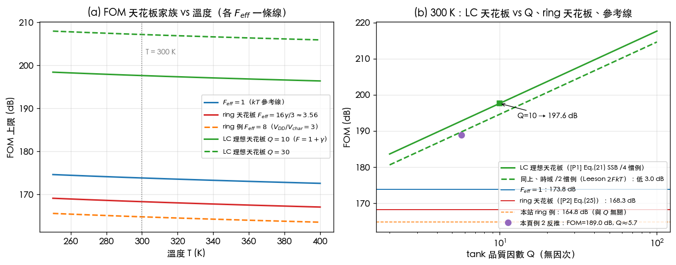
• Script: simulations/fig_fom_limit.py (run with PYTHONPATH=. python3 simulations/fig_fom_limit.py, which prints all the key numbers on this page and saves the figure).
• Parameters: $k=1.380649\times10^{-23}$ J/K; ring: $\eta=1$, $\gamma=2/3$, $V_{DD}/V_{char}\in\{2\gamma,3\}$; LC: $F=1+\gamma$, $\Gamma_{rms}^2=\tfrac12$, $\eta_P=1$, $Q\in[2,100]$.
• How to read it: (a) each line is a $F_{eff}$ ceiling's trend vs. temperature $T$ (slope $\approx-0.14$ dB/10 K); (b) the green line is the ideal LC ceiling vs. $Q$ (solid /4, dashed /2 convention), and the horizontal lines from top to bottom are the reference line 173.8, the ring ceiling 168.3, and this site's ring example 164.8. The figure deliberately omits a scatter of published designs — none of the five source PDFs contains verifiable per-design FOM data, so drawing lines without points is the honest approach (the purple dot and green square are examples computed on this page).

How many dB below the ceiling?

• Good published LC designs: survey-table standouts commonly fall in the $188\sim195$ dB range (order-of-magnitude statement; corresponding to $F_{eff}\approx0.008\sim0.03$, which can be back-derived from this page's bound family, e.g. worked example 2's $189$ dB → an equivalent $Q\approx5.7$). Against their own $Q$-based ceiling ($Q=10\sim15$ → $197.6\sim201.2$ dB, /4 convention), the typical gap is about $5\sim10$ dB — eaten by $\eta_P\lt1$, tail/bias noise ($F\gt1+\gamma$), varactor/switch loss (lowering effective $Q$), and layout parasitics. In other words: the LC problem has already been solved to within arm's reach of the physical limit, and every remaining dB costs more than the last.
• Colpitts vs. LC-tank (Andreani et al., JSSC 2005; external literature, not among the five source PDFs, full citation at page bottom): this paper gives closed-form noise factors for CMOS Colpitts and differential LC-tank oscillators and validates them experimentally, with the well-known conclusion that in CMOS, LC-tank phase-noise performance is at least as good as Colpitts's — Colpitts's cyclostationary advantage (current pulse aligned to the ISF trough; this site's real_oscillator_topologies example 2 estimates roughly a 7 dB reduction in $\Gamma_{eff,rms}^2$) is offset by its bias-efficiency and startup-margin cost. Both topologies sit under the same LC ceiling family (both have an $F$ from the $1+\gamma$ family and a $1/Q^2$ term) — neither can bypass the wall set by $Q$.
• Ring: this site's example sits only $3.5$ dB below the ring ceiling — the ring's universal form has no $Q$ to buy with, and the ceiling itself (168.3 dB) is already about 30 dB below LC's.

Ring's dB deficit vs. LC, itemized (this site's ring example at 164.8 dB against the LC ideal ceiling at $Q=10$, 197.63 dB, a gap of $32.83$ dB; fig_fom_limit.py verifies the itemized terms sum exactly to the total gap):

Term	Ratio	dB	Physics
No energy storage vs. $2Q^2$ ($Q=10$)	$200$	$23.0$	LC's high-$Q$ storage beats down $kT$; the ring discards all its energy and recharges every cycle
$V_{DD}/V_{char}=3$	$3$	$4.8$	Overdrive/headroom: smaller $V_{char}$ amplifies more noise
Leading coefficient $8/3$	$8/3$	$4.3$	Ring waveform/transition bookkeeping ([P2] Eq.(23)'s $8/(3\eta)$)
LC waveform term $(1+\gamma)\Gamma_{rms}^2$	$5/6$	$0.8$	LC's own $F$ and $-\sin$ ISF claw back only a little
Total	$1920$	$32.8$	$=197.63-164.80$ ✓

Actual published LC designs don't hit their ideal ceiling (they give back $5\sim10$ dB), so the observed real-world gap is about 25 dB — consistent with "good LC $\approx190$, good ring $\approx165$." Conclusion: the ring's deficit is not a lack of design effort — it's a structural gap made of $Q$ (the 23 dB term) plus $V_{char}$/waveform (about 9 dB); the ring's selling points are area, tuning range, and multi-phase output (see lc_vs_ring).

Worked examples

Example 1 (converting this site's ring example to FOM, and locating it relative to the ceiling) Given lc_vs_ring example 1: $\mathcal{L}=-91.0$ dBc/Hz @ $\Delta f=1$ MHz, $f_0=5$ GHz, $P=1$ mW. Find FOM and the distance to the ring ceiling.

Step-by-step substitution (with units):

$$\begin{aligned} 20\log_{10}\!\left(\frac{f_0}{\Delta f}\right)&=20\log_{10}\!\left(\frac{5\times10^9\ \text{Hz}}{10^6\ \text{Hz}}\right)=20\log_{10}(5000)=73.98\ \text{dB},\\[4pt] 10\log_{10}\!\left(\frac{P}{1\ \text{mW}}\right)&=10\log_{10}(1)=0\ \text{dB},\\[4pt] \mathrm{FOM}&=-(-91.0)+73.98-0=164.98\approx165.0\ \text{dB}. \end{aligned}$$

• Result: $\mathrm{FOM}\approx165$ dB; about $3.5$ dB below the ring ceiling at $168.3$ dB (entirely from $V_{DD}/V_{char}=3$ vs. the lower bound $2\gamma=4/3$), and $9.0$ dB below the reference line at $173.8$ dB ($F_{eff}=8$).
• Dimension check: all three terms are logs of dimensionless ratios → dB ✓ ($f_0/\Delta f$: Hz/Hz; $P/1$ mW: W/W).
• One-line Python check:

import numpy as np
print(round(91.0 + 20*np.log10(5e9/1e6) - 10*np.log10(1e-3/1e-3), 2))   # -> 164.98

Example 2 (design back-derivation: reading an "equivalent $Q$" off a measured FOM) An $f_0=5$ GHz LC VCO burns $P=10$ mW and measures $\mathcal{L}(1\ \text{MHz})=-125$ dBc/Hz. Find FOM, the implied $F_{eff}$, and, assuming $F=2$, $\Gamma_{rms}^2=\tfrac12$, $\eta_P=0.5$ (a more realistic loss assumption), the implied tank $Q$.

Step-by-step substitution (with units):

$$\begin{aligned} \mathrm{FOM}&=125+20\log_{10}(5000)-10\log_{10}(10)=125+73.98-10=188.98\ \text{dB},\\[4pt] F_{eff}&=10^{(C_{ref}-\mathrm{FOM})/10}=10^{(173.83-188.98)/10}=10^{-1.515}=0.0305,\\[4pt] Q&=\sqrt{\frac{F\,\Gamma_{rms}^2}{2\,F_{eff}\,\eta_P}} =\sqrt{\frac{2\times0.5}{2\times0.0305\times0.5}}=\sqrt{32.7}=5.72 . \end{aligned}$$

• Result: $\mathrm{FOM}=189.0$ dB — a "good design" figure; the implied $Q\approx5.7$ is entirely reasonable on-chip. If the process could give $Q=10$ (ideal ceiling $197.6$ dB, /4 convention), this design would sit about $8.7$ dB below its own ceiling — the next thing to check is $\eta_P$ (class efficiency), tail noise ($F$), and varactor loss, not piling on more current.
• Dimension check: $F_{eff}$ dimensionless (dB difference ÷10 then exponentiated) ✓; everything under the square root is dimensionless → $Q$ dimensionless ✓.
• One-line Python check:

import numpy as np
Cref = -10*np.log10(1.380649e-23*300/1e-3)
FOM = 125.0 + 20*np.log10(5e9/1e6) - 10*np.log10(10e-3/1e-3)
print(round(FOM, 2))                           # -> 188.98
Feff = 10**((Cref - FOM)/10)
print(round(Feff, 4))                          # -> 0.0305
print(round(np.sqrt(2*0.5/(2*Feff*0.5)), 2))   # -> 5.72 (implied Q; F=2, Γrms²=0.5, η_P=0.5)

Design knobs: what moves FOM, what doesn't

Knob	What it moves	Effect	Note
Raise tank $Q$	$F_{eff}^{LC}\propto1/Q^2$	$+20$ dB per decade of $Q$ ($+6$ dB per doubling of $Q$)	The only big lever; limited by process inductor/varactor quality
Raise power efficiency $\eta_P$ (class-B→C/D/F)	$1/\eta_P$	A few dB at most	Swing waveform and conduction-angle engineering
Reduce $F$ (tail filter, symmetry, clean bias)	$F\to1+\gamma$	A few dB	Hegazi 2001 (external literature) family of techniques
Waveform/ISF engineering	$\Gamma_{rms}^2$	On the order of $1\sim2$ dB	class-F, harmonic shaping
Add power $P$	—	0 dB	FOM is already normalized to $P$; only lowers $\mathcal{L}$, not FOM
Ring: add stages $N$	—	0 dB	[P2] N-independence; $N$ doesn't appear in Eq.(23)
Cool down	$C_{ref}(T)$	$+0.14$ dB per $-10$ K	Usually not something you get to choose
Ring's $V_{DD}/V_{char}$	$F_{eff}^{ring}$	Up to the $2\gamma$ lower bound (a $\sim3.5$ dB gap)	Beyond that you hit the [P2] Eq.(25) ceiling

Connection to SerDes

The FOM ceiling translates directly into "the lowest jitter buyable within a given power budget." Example C (lab_08: $f_0=5$ GHz, $-100$ dBc/Hz @ 1 MHz, $1/f^2$, integrated 1–100 MHz) gives $\sigma_t=447.9$ fs; by the same method $\sigma_t\propto10^{\Delta\mathcal{L}/20}$, so a 1 mW, 165-dB-FOM ring ($-91$ dBc/Hz, 9 dB higher than example C) gives:

print(round(447.9 * 10**((100.0-91.0)/20), 1))   # -> 1262.4 (fs; same integration bandwidth, same 1/f² slope)

about $1.26$ ps rms — unusable for $\ge56$ Gb/s SerDes UIs, which is why high-speed SerDes only trusts LC-PLL plus (when needed) ring in positions suppressed within the PLL bandwidth (see serdes_clocking_connection, pll_noise_budget).

Applicability and breakdown conditions

Condition	When it holds	When it breaks down
Offset in the $1/f^2$ white-noise region	The universal form and $\mathrm{FOM}=173.8-10\log_{10}F_{eff}$ hold	In the $1/f^3$ (flicker) region or the floor region: FOM changes with $\Delta f$, making comparison meaningless
$P$ = total DC power dissipation	Fair cross-design comparison	Reporting only core power (omitting buffer/bias) inflates FOM
$T=300$ K	Constant $173.83$ dB	Other temperatures use $C_{ref}(T)$ ($-0.14$ dB/10 K)
Theoretical value states /2 or /4 convention	Ceilings can be cross-compared (differ by $3.01$ dB)	Mixing conventions produces a phantom 3 dB
Small-perturbation LTV ([P1] framework)	$F_{eff}$ is constant	Large injection, injection pulling (see the [P3]/[P4] pages) require separate treatment
Looking at FOM alone	Normalizes the power–noise trade-off	Area, tuning range (the FOM$_T$ variant covers this separately), supply pushing, yield are all outside its scope

Key takeaways

• $\mathrm{FOM}=-\mathcal{L}+20\log_{10}(f_0/\Delta f)-10\log_{10}(P/1\text{mW})$ (this page's positive-value convention; tank_swing uses its negative). By construction, $(f_0/\Delta f)^2$ and $P$ cancel exactly.
• Universal reduction: $\mathcal{L}_{lin}=F_{eff}(kT/P)(f_0/\Delta f)^2\Rightarrow\mathrm{FOM}=173.8-10\log_{10}F_{eff}$ dB (300 K). The constant $173.83=-10\log_{10}(kT\cdot1\text{Hz}/1\text{mW})$ pairs with 1·kT ($2kT$ pairs with $170.8$ — don't mix them up); every factor-of-2 convention lives inside $F_{eff}$ (/2 vs. /4 = 3.01 dB).
• Ring: $F_{eff}=(8/(3\eta))(V_{DD}/V_{char})\ge16\gamma/(3\eta)$ ([P2] Eq.(23)/(25)) → ceiling $168.3$ dB; this site's $-91$ dBc/Hz example = $165$ dB, only $3.5$ dB below the top.
• LC: $F_{eff}=F\Gamma_{rms}^2/(2Q^2\eta_P)$ (derived from [P1] Eq.(21)) → ceiling rises with $Q$: $Q=10$ gives $197.6$ dB (/4) / $194.6$ dB (/2). $Q$ is the only big lever.
• Good published LC designs ($\approx190$ dB) sit about $5\sim10$ dB below their own $Q$ ceiling; ring trails LC by about 25 dB, itemized as: energy storage $2Q^2$ (23 dB) + $V_{char}$/waveform ($\sim9$ dB).
• The ceiling is a family, not a magic number — when citing any "FOM limit," first ask what $F_{eff}$ ($\gamma$, $Q$, $\eta_P$, convention) it assumes.

Further reading

• FOM definition and the phase-noise × power trade-off: tank_swing
• [P1] Eq.(21) derivation and the /2 vs. /4 convention: white_noise_to_phase_noise
• [P2] ring FOM and N-independence: lc_vs_ring, paper_002 deep-dive
• Leeson's $2FkT/P_s$ compared against ISF: derivation_leeson
• Where topology-level $F$ comes from (tail, Colpitts narrow window): real_oscillator_topologies
• The FOM → jitter → BER chain: serdes_clocking_connection, lab_08
• Site-wide citation list: references

External literature (not among the five downloaded source PDFs)

• [E-Hegazi] E. Hegazi, H. Sjöland, and A. A. Abidi, "A Filtering Technique to Lower LC Oscillator Phase Noise," IEEE J. Solid-State Circuits, vol. 36, no. 12, pp. 1921–1930, Dec. 2001. (LC noise-factor lower bound $F\to1+\gamma$ and the tail filter; already cited and verified by volume/page on this site in tank_swing.)
• [E-Andreani] P. Andreani, X. Wang, L. Vandi, and A. Fard, "A Study of Phase Noise in Colpitts and LC-Tank CMOS Oscillators," IEEE J. Solid-State Circuits, vol. 40, no. 5, pp. 1107–1118, May 2005. (Closed-form noise factors and measured comparison for Colpitts vs. LC-tank; already cited on this site in real_oscillator_topologies, DOI 10.1109/JSSC.2005.845991. This page only draws on its abstract-level conclusion and does not transcribe its internal formulas.)
• [E1] Leeson 1966: D. B. Leeson, "A Simple Model of Feedback Oscillator Noise Spectrum," Proc. IEEE, vol. 54, no. 2, pp. 329–330, Feb. 1966. (The $2FkT/P_s$ form; see derivation_leeson.)
• [E-Friis] H. T. Friis, "Noise Figures of Radio Receivers," Proc. IRE, vol. 32, no. 7, pp. 419–422, Jul. 1944. (Origin of the $T_0=290$ K noise-reference-temperature convention; $-174$ dBm/Hz is the $kT_0$ conversion.)