β: This English translation is in beta — the Traditional-Chinese original is the authoritative version.

Leeson Model Derivation and ISF Comparison

Prerequisites / See also: tank_Q_and_energy_restoration (the energy definition of $Q$, why the tank shapes $1/f^2$), psd_phase_noise_jitter ($4kTR$ thermal noise and PSD basics), white_noise_to_phase_noise (the ISF-version $1/f^2$ derivation) | Next: symmetry (using $c_0$ symmetry to suppress the $1/f^3$ corner), references (external literature [E1])

Before Hajimiri–Lee's ISF theory ([P1], 1998) appeared, engineers estimated oscillator phase noise using the Leeson model (1966). It is a semi-empirical formula: the physical skeleton (tank filtering + feedback) is correct, but it packs in a noise factor $F$ that is "unknown where it comes from — has to be fit from measurement." This page derives Leeson from scratch, then maps it term by term onto the closed-form ISF result — you'll see that ISF theory "explains why Leeson looks the way it does, and replaces that mysterious $F$ with a computable physical quantity."

Honesty note (read first): the Leeson model comes from [E1] D. B. Leeson, "A Simple Model of Feedback Oscillator Noise Spectrum," Proc. IEEE, vol. 54, no. 2, pp. 329–330, Feb. 1966, not among the five source PDFs downloaded for this site. This page relies only on standard-literature knowledge for background and comparison; the volume/issue/pages/DOI have been verified online (DOI 10.1109/PROC.1966.4682); $F$ (noise figure) is inherently an empirically fitted parameter of the Leeson model (implementation-dependent), not a fixed constant. By contrast, the ISF formulas in the right half of this page ([P1] Eqs.(21),(23),(24)) are authoritative, verified expressions from within the five source PDFs.

This page answers:

1. Physically, where does each term of the Leeson expression (floor, $1/f^2$, $1/f^3$) come from?
2. Why are the slopes $1/f^2$ and $1/f^3$, and where is the corner?
3. Which ISF quantities do Leeson's $Q$, $F$, $\omega_{1/f^3}$ correspond to? Which ones does ISF explain more clearly?

Physical intuition (conclusion first): Leeson treats the oscillator as "a feedback system continuously fed by thermal noise and narrowband-filtered by a high-$Q$ tank." Three things stack up: (1) the amplifier/tank injects a white noise floor ($2FkT/P_s$); (2) because it is an autonomous oscillator, phase perturbations near the carrier have no restoring force, so the closed loop multiplies the noise by a $(\omega_0/2Q\Delta\omega)^2$ "phase-integration" transfer function, producing the $1/f^2$ skirt; (3) the device's $1/f$ flicker noise gets upconverted by one more order, producing the $1/f^3$ closest to the carrier. ISF theory tells the same three-part story, only it replaces $1/2Q$ with $\Gamma_{rms}/q_{max}$, and replaces $F$ with a physical quantity computable from $\Gamma_{eff}$.

The full formula (state it first, then derive step by step)

Leeson model (spec 10.2, external literature, not one of the five PDFs):

$$\mathcal{L}(\Delta\omega)=10\log_{10}\!\left[\frac{2FkT}{P_s}\left(1+\Big(\frac{\omega_0}{2Q\,\Delta\omega}\Big)^2\right)\left(1+\frac{\omega_{1/f^3}}{\lvert\Delta\omega\rvert}\right)\right]$$

Symbols: $F$ = amplifier noise figure (empirical quantity, dimensionless); $k$ = Boltzmann constant (J/K); $T$ = temperature (K); $P_s$ = oscillation signal power (W); $Q$ = tank quality factor (dimensionless); $\omega_0$ = carrier angular frequency (rad/s); $\Delta\omega$ = offset angular frequency (rad/s); $\omega_{1/f^3}$ = flicker corner (rad/s).

Below, the three factors inside the brackets are derived one at a time.

Step 1: tank thermal noise — the noise floor $2FkT/P_s$

Treat the oscillator as a "feedback loop of amplifier + resonant tank." The thermal-noise source in the loop is the tank's loss resistance $R$ (parallel-equivalent), whose single-sided thermal-noise voltage PSD (Johnson–Nyquist) is:

$$\frac{\overline{v_n^2}}{\Delta f}=4kTR.$$

• Physics used: resistor thermal noise $4kTR$ (standard result; see psd_phase_noise_jitter).
• Dimension check: $[kT]=\text{J}=\text{V·C}$, $[kTR]=\text{V·C·}\Omega=\text{V}^2\text{·s}=\text{V}^2/\text{Hz}$ ✓.

The amplifier itself also adds noise; the whole thing is lumped into a single noise figure $F$ (which packages "actual total noise" over "input thermal noise alone" into one ratio). Normalizing the noise power against the carrier power $P_s$ gives the phase-noise floor near the carrier:

$$\mathcal{L}_{\text{floor}}=\frac{2FkT}{P_s}.$$

• $F$ is Leeson's "empirical escape hatch": it absorbs all the noise that isn't explicitly modeled (amplifier, conversion loss, cyclostationary effects, ...) into a single measurement-fit number. This is exactly what ISF later replaces (see Step 5's comparison).
• Where the 2 comes from: this is a bookkeeping convention of the Leeson model (not the only way to write it — it varies by reference). Physically there are actually two factors, pulling in opposite directions: (1) AM/PM equipartition — thermal noise perturbs amplitude and phase simultaneously, and phase gets only half the power ($\times\tfrac12$); (2) single-sideband (SSB) accounting converts double-sided power to single-sided ($\times2$). The two cancel, so the "cleanest" way to write the floor is actually $FkT/P_s$; writing it as $2FkT/P_s$ leaves the SSB convention explicit in the leading constant without folding the AM/PM $\tfrac12$ into $F$. This is the same kind of SSB/double-sided bookkeeping difference as [P1] Eq.(21)'s $4\Delta\omega^2$ vs. the time-domain $2\Delta\omega^2$ (see the factor-of-2 discussion in white_noise_to_phase_noise). ($F$ is an empirically fitted parameter, and the leading constant varies slightly by reference — this is precisely what ISF later replaces with $\Gamma_{rms}/q_{max}$.)
• Dimension check: $[2FkT/P_s]=\text{J}/\text{W}=\text{J}/(\text{J/s})=\text{s}=1/\text{Hz}$ ✓ ($\mathcal{L}$ is relative power per hertz, dBc/Hz).

Step 2: narrowband filtering by the high-$Q$ tank → the $1/f^2$ skirt

The tank is a narrowband filter. Near the carrier, at offset $\Delta\omega$, the phase/amplitude response slope of the parallel RLC is set by $Q$. The standard result: the (half-power) transfer of the tank at offset $\Delta\omega$ can be written as

$$\left|H(\Delta\omega)\right|^2\;\propto\;\left(\frac{\omega_0}{2Q\,\Delta\omega}\right)^2\qquad(\Delta\omega\ll\omega_0/2Q).$$

• The physics of $Q$: $Q=\omega_0/\Delta\omega_{3dB}$ = "how sharp the resonance peak is" = stored/dissipated energy ratio per cycle $\times2\pi$. The higher the $Q$, the narrower the tank bandwidth, the steeper the phase slope, and the stronger the suppression of offset noise.
• Why $1/\Delta\omega^2$ (i.e., $-20$ dB/dec): an autonomous oscillator's phase is a neutral direction (no restoring force, echoing $\lambda_1=0$ in derivation_floquet_ppv). The closed loop is equivalent to one integration of the phase perturbation, which in the frequency domain is $\times 1/\Delta\omega$; squaring for power gives $1/\Delta\omega^2$. This is the fundamental reason phase noise must be $1/f^2$ in the mid-band, slope $-20$ dB/dec — it shares the same origin as ISF's $1/\Delta\omega^2$ ([P1] Eq.(21)).
• Dimension check: $\omega_0/(2Q\Delta\omega)$ is dimensionless (rad/s ÷ rad/s) ✓, so the whole transfer is dimensionless.

Multiplying Steps 1 and 2 (floor × tank shaping) gives the first two terms in the brackets:

$$\mathcal{L}_{1/f^2+\text{floor}}=\frac{2FkT}{P_s}\left(1+\Big(\frac{\omega_0}{2Q\,\Delta\omega}\Big)^2\right).$$

• The $1$ in "$1+$" is the white noise floor (dominant at far offset, flat); $(\omega_0/2Q\Delta\omega)^2$ is the $1/f^2$ skirt (dominant near the carrier). Where the two are equal is the corner where $1/f^2\to$ floor, $\Delta\omega\approx\omega_0/2Q$.

Step 3: device flicker → the $1/f^3$ region closest to the carrier

The device's low-frequency $1/f$ (flicker) noise gets "upconverted" near the carrier by the oscillator's nonlinearity, and after the phase integration of Step 2, becomes a $1/f^3$ steeper than $1/f^2$. Leeson attaches it with a multiplicative factor:

$$\left(1+\frac{\omega_{1/f^3}}{\lvert\Delta\omega\rvert}\right).$$

• When $\Delta\omega\gg\omega_{1/f^3}$: this factor $\approx1$, flicker is invisible, leaving just $1/f^2$ and the floor.
• When $\Delta\omega\ll\omega_{1/f^3}$: this factor $\approx\omega_{1/f^3}/\lvert\Delta\omega\rvert\propto1/\Delta\omega$, which further multiplies the $1/\Delta\omega^2$ from Step 2 → total $1/\Delta\omega^3$, i.e., $1/f^3$, $-30$ dB/dec.
• $\omega_{1/f^3}$ is the "flicker corner of the phase noise", not the device's own $1/f$ corner. Leeson never explains what determines it — this is exactly the key physics ISF fills in (Step 5, [P1] Eq.(24)).
• Dimension check: $\omega_{1/f^3}/\lvert\Delta\omega\rvert$ dimensionless ✓.

Multiplying all three terms gives the full Leeson formula from the top. Three slope segments: floor (flat) → $1/f^2$ ($-20$ dB/dec) → $1/f^3$ ($-30$ dB/dec), from far to near.

Step 4: Leeson vs ISF overlay

Plotting the Leeson formula and the ISF result ([P1] Eqs.(21),(23),(24)) on the same log–log axes, the three segments ($1/f^3$, $1/f^2$, floor) overlap — the two models describe the same curve, just with different physical meanings assigned to the parameters:

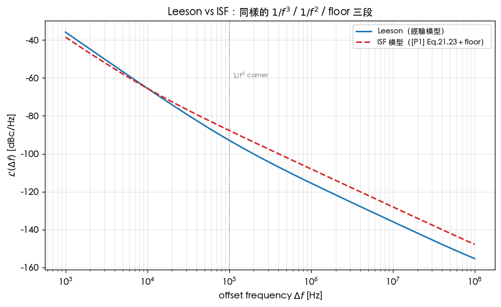
• Formula correspondence: left half is the Leeson expression from the top (external literature); right half is [P1] Eq.(21) ($1/f^2$), Eq.(23) ($1/f^3$), Eq.(24) ($1/f^3$ corner).
• script / function: simulations/lab_16_leeson_vs_isf.py (main), corresponding to leeson_vs_isf_overlay.png in the spec 10.1 table (lab_16). This is a pedagogical toy model, not transistor-level; the Leeson curve is drawn illustratively for the $1/f^2$ segment using functions like leeson_one_over_f2 from simulations/common/noise_utils.py, and the constants used to stitch the three segments are for teaching illustration only.
• How to read it: the two curves are exactly parallel in the mid-band $1/f^2$ region (both slope $-20$ dB/dec, since both come from "phase integration $1/\Delta\omega^2$"); near the carrier both turn into $1/f^3$; far out both flatten to the floor. The only difference is where the corner falls and the absolute level — which is set by the parameter correspondence, see below.
• Note: in the overlay, the Leeson segment's $F,Q,\omega_{1/f^3}$ and the ISF segment's $\Gamma_{rms},q_{max},c_0,\omega_{1/f}$ are illustrative teaching values (lab_16 parameters), used to show the three-segment slope overlap, not measurements of a specific circuit.

Step 5: term-by-term comparison (Leeson ↔ ISF)

This is the core of this page. Putting the corresponding terms of both models side by side:

Segment	Leeson (empirical, [E1] 1966, not one of the five PDFs)	ISF ([P1] 1998, within the five PDFs)	Correspondence and where "ISF is clearer"
$1/f^2$ shaping	$\Big(\dfrac{\omega_0}{2Q\,\Delta\omega}\Big)^2$	$\dfrac{\Gamma_{rms}^2}{q_{max}^2}\cdot\dfrac{1}{\Delta\omega^2}$ ([P1] Eq.(21))	Both give $1/\Delta\omega^2$. Leeson's $\dfrac{1}{2Q}$ ↔ ISF's $\dfrac{\Gamma_{rms}}{q_{max}}\times$ (including carrier/noise-power normalization). $Q$↔$\Gamma_{rms}/q_{max}$: high $Q$ = low $\Gamma_{rms}/q_{max}$ = low phase noise.
Noise source/level	$\dfrac{2FkT}{P_s}$, $F$ empirically fit	$\dfrac{\overline{i_n^2}/\Delta f}{4}$ paired with $\Gamma_{eff}$ (including cyclostationary)	Empirical $F$ vs ISF physical: Leeson's $F$ is "you only know it once you measure it"; ISF splits it into a computable device noise PSD × $\Gamma_{eff}$, which can even fold in cyclostationary gating (see effective_isf).
$1/f^3$ corner	$\omega_{1/f^3}$ (Leeson never says what sets it)	$\Delta\omega_{1/f^3}=\omega_{1/f}\dfrac{c_0^2}{2\Gamma_{rms}^2}\approx\omega_{1/f}\Big(\dfrac{c_0}{c_1}\Big)^2$ ([P1] Eq.(24))	ISF's signature insight: the $1/f^3$ corner is not equal to the device's own $1/f$ corner $\omega_{1/f}$, but is scaled by $(c_0/\Gamma_{rms})^2$. Waveform symmetry → $c_0\to0$ → corner pushed far below $\omega_{1/f}$. Leeson gives no visibility into this design lever at all.

Key comparisons expanded:

(a) $Q\leftrightarrow\Gamma_{rms}/q_{max}$. Both are "the efficiency with which noise is converted into a phase skirt." Leeson says "higher $Q$ is better"; ISF says "smaller $\Gamma_{rms}/q_{max}$ is better." But ISF is more general: it also holds for ring oscillators with no high-$Q$ tank (a ring has no $Q$ to speak of, but does have $\Gamma_{rms},q_{max}$; see lab_03). This is the first way ISF goes beyond Leeson.

(b) Empirical $F$ vs ISF physical. Leeson's $F$ is a black box: you must first build the oscillator, measure the phase noise, and back out $F$, before you can "predict" with the model — which is really post-hoc fitting, not prediction. ISF writes the same level as $\dfrac{\overline{i_n^2}/\Delta f}{4q_{max}^2}\Gamma_{rms}^2$ ([P1] Eq.(21)), where every quantity can be computed ahead of time from the device model and waveform, and cyclostationary behavior (device leaking noise only at certain phases) can be folded in via $\Gamma_{eff}=\Gamma\cdot\alpha$ — this is exactly why the Colpitts's "effective $F$" is much lower than a naive Leeson estimate (see effective_isf).

(c) $1/f^3$ corner. Leeson simply takes $\omega_{1/f^3}$ as an input parameter, effectively admitting "I don't know where it comes from." Early engineering practice even mistook it for the device's own $1/f$ corner. ISF's [P1] Eq.(24) settles it: $\Delta\omega_{1/f^3}=\omega_{1/f}\cdot c_0^2/(2\Gamma_{rms}^2)$ — it is set by the ISF's DC coefficient $c_0$ (waveform symmetry). Making rise/fall symmetric → $c_0\to0$ → the $1/f^3$ corner drops sharply → near-carrier phase noise falls substantially. This is a design rule Leeson simply cannot give, and it is the theoretical basis for [P2]'s use of symmetry to suppress ring phase noise (see symmetry, flicker_noise_upconversion).

Numerical example (building intuition)

Example ($1/f^3$ corner comparison): take a device $1/f$ corner $f_{1/f}=1$ MHz ($\omega_{1/f}=2\pi\times10^6$ rad/s). Compare the phase-noise $1/f^3$ corner of a "symmetric" vs. an "asymmetric" waveform.

ISF's [P1] Eq.(24): $\Delta\omega_{1/f^3}=\omega_{1/f}\cdot c_0^2/(2\Gamma_{rms}^2)$, take $\Gamma_{rms}=0.5$.

• Asymmetric waveform (large $c_0$, set $c_0=0.4$):

$$\Delta\omega_{1/f^3}=\omega_{1/f}\cdot\frac{(0.4)^2}{2(0.5)^2}=\omega_{1/f}\cdot\frac{0.16}{0.5}=0.32\,\omega_{1/f}.$$

That is, $f_{1/f^3}\approx0.32\times1\ \text{MHz}=320$ kHz — the $1/f^3$ skirt extends far from the carrier.

• Symmetric waveform (small $c_0$, set $c_0=0.04$, 10× smaller):

$$\Delta\omega_{1/f^3}=\omega_{1/f}\cdot\frac{(0.04)^2}{2(0.5)^2}=\omega_{1/f}\cdot\frac{0.0016}{0.5}=3.2\times10^{-3}\,\omega_{1/f}.$$

That is, $f_{1/f^3}\approx3.2$ kHz — the corner drops 100× (because $c_0$ is squared: a 10× reduction in $c_0$ → 100× reduction in the corner).

• Dimension check: $c_0^2/\Gamma_{rms}^2$ is dimensionless, $\omega_{1/f}\times$dimensionless $=$ rad/s ✓.
• Intuition: Leeson treats $\omega_{1/f^3}$ as "fixed by nature"; ISF tells you it is a knob the designer can turn by two orders of magnitude via symmetry. This is ISF's practical value.

One-line Python verification (corner ratio):

import numpy as np
from simulations.common.isf_utils import gamma_rms
# Ratio of the 1/f^3 corner for a symmetric vs asymmetric waveform = (c0_asym/c0_sym)^2
c0_asym, c0_sym, Gamma_rms = 0.4, 0.04, 0.5
w1f = 2*np.pi*1e6
corner_asym = w1f * c0_asym**2 / (2*Gamma_rms**2)
corner_sym  = w1f * c0_sym**2  / (2*Gamma_rms**2)
print(corner_asym/(2*np.pi)/1e3, "kHz ;", corner_sym/(2*np.pi)/1e3, "kHz")
# -> ~320.0 kHz ; ~3.2 kHz   (a symmetric waveform pushes the 1/f^3 corner down 100x)

(For gamma_rms and related library functions, see simulations/common/isf_utils.py; this example computes the corner directly by hand from [P1] Eq.(24).)

Applicability and failure conditions

Condition	When Leeson holds	What happens when it fails
High-$Q$ resonant tank present	$(\omega_0/2Q\Delta\omega)^2$ shaping is accurate	No-$Q$ topologies like ring don't apply → use ISF's $\Gamma_{rms}/q_{max}$ instead
$F$ obtainable by measurement fit	Curve can be fit post-hoc	Want to predict ahead of time or decompose the physics → must use ISF ($F$ is a black box)
$\omega_{1/f^3}$ known	$1/f^3$ segment matches	Want to know what sets the corner / how to suppress it → ISF Eq.(24) ($c_0$, symmetry)
Linear/weakly nonlinear, additive noise	Three-segment model suffices	Strongly cyclostationary → only ISF's $\Gamma_{eff}=\Gamma\alpha$ gets it right

Corresponding papers/equations

• The Leeson model itself: [E1] D. B. Leeson, Proc. IEEE 54(2):329–330, Feb. 1966 — not among the five downloaded source PDFs; volume/DOI verified (10.1109/PROC.1966.4682, see [E1] in references); this formula is the standard Leeson form ($F$ is an empirical noise factor, leading constant varies slightly by reference).
• ISF comparison equations (within the five PDFs, verified): $1/f^2$ [P1] Eq.(21), p.185; $1/f^3$ [P1] Eq.(23), p.185; $1/f^3$ corner [P1] Eq.(24), p.185; device flicker [P1] Eq.(22), p.185.
• Cyclostationary (explaining "effective $F$"): [P1] Eqs.(25)–(27), p.186 (see effective_isf).
• Overlay plot: /figures/leeson_vs_isf_overlay.png, simulations/lab_16_leeson_vs_isf.py (spec 10.1, lab_16).

Key takeaways

• Leeson (1966, external, not one of the five PDFs) = a semi-empirical three-term expression: $\mathcal{L}=10\log_{10}\!\big[\tfrac{2FkT}{P_s}(1+(\tfrac{\omega_0}{2Q\Delta\omega})^2)(1+\tfrac{\omega_{1/f^3}}{\lvert\Delta\omega\rvert})\big]$.
• Three segments: white-noise floor ($2FkT/P_s$) → tank-shaped $1/f^2$ ($-20$ dB/dec, from phase integration $1/\Delta\omega^2$) → flicker-upconverted $1/f^3$ ($-30$ dB/dec).
• Term-by-term correspondence: $Q\leftrightarrow\Gamma_{rms}/q_{max}$ (high $Q$ = low $\Gamma_{rms}/q_{max}$); empirical black-box $F$ ↔ ISF's computable $\overline{i_n^2}\cdot\Gamma_{eff}$ (including cyclostationary); mysterious parameter $\omega_{1/f^3}$ ↔ [P1] Eq.(24), set by $c_0$ (symmetry).
• ISF's three big advances: (1) also holds for no-$Q$ rings; (2) computable ahead of time, not fit-dependent; (3) turns the $1/f^3$ corner into a design knob that symmetry can move by two orders of magnitude.
• The two models overlap on all three segments in a log–log plot (leeson_vs_isf_overlay.png) — the same curve, different physical languages.

Further reading

• $1/f^2$ white-noise derivation (ISF version): white_noise_to_phase_noise
• $1/f^3$ flicker upconversion and corner: flicker_noise_upconversion
• How symmetry suppresses $c_0$: symmetry
• "Effective $F$" and cyclostationary: effective_isf
• PSD / phase noise / jitter basics: psd_phase_noise_jitter
• Rigorous foundation (PPV/Floquet): derivation_floquet_ppv
• Full bibliography and external citations ([E1]): references