β: This English translation is in beta — the Traditional-Chinese original is the authoritative version.

Rigorous LTV framework: Zadeh's time-varying transfer function and the harmonic transfer matrix

Prerequisites: lti_vs_ltv (intuition for LTV vs. LTI), convolution_derivation ([P1] Eq.(11)'s LTV convolution), fourier_series_of_isf (ISF Fourier coefficients $c_n$) | Next: derivation_floquet_ppv (the PPV/Floquet face of the same ISF)

This site's main thread ([P1]) introduces the ISF via "physical intuition + impulse simulation," and convolution_derivation uses superposition to generalize a single impulse to arbitrary noise. That path works very well, but leaves a gap: we keep saying the oscillator's response to noise is LTV (linear time-varying), "it acts like a time-varying mixer that shifts noise near $n\omega_0$ to the carrier" — but in the language of signals and systems, exactly which rigorous object do these statements correspond to? Can "frequency gets shifted, gain is $c_k$" be written as a clean transfer function?

This page fills in that system-theory foundation. Starting from the convolution/LTI framework the reader already knows, we work up to Zadeh's time-varying transfer function $H(f,t)$ and the harmonic transfer matrix (HTM), and then prove one statement:

The ISF (together with $1/q_{max}$) is exactly the "conversion vector from each input-harmonic band to the phase output" — its $k$-th component is precisely the $k$-th Fourier coefficient $c_k$ of the ISF. In other words, the ISF's Fourier series $\{c_k\}$ is not merely a set of numbers — it is exactly the "phase-output row" of this LTV system's HTM.

Honesty note (read first): this page's Zadeh time-varying transfer function $H(f,t)$, bi-frequency function, and harmonic transfer matrix (HTM) belong to the broader theory of linear time-varying systems and are not among the 5 PDFs hosted on this site. The original concept comes from [E5] L. A. Zadeh, "Frequency Analysis of Variable Networks," Proc. IRE, vol. 38, no. 3, pp. 291–299, Mar. 1950 (DOI 10.1109/JRPROC.1950.231083); the HTM formulation is standard in periodic-time-varying/RF circuit literature (e.g., cyclostationary, LPTV system analysis). These are external mathematical frameworks; the formal [E5] citation (Zadeh 1950, Proc. IRE 38(3):291–299, DOI 10.1109/JRPROC.1950.231083) is recorded in references. This page only uses them to "re-derive the ISF"; every correspondence to the ISF converges back to [P1] Eq.(13) (within the 5 PDFs, verified verbatim).

This page answers four questions:

1. How does LTI convolution generalize to LTV? (First connect to the reader's signals-and-systems background.)
2. How does Zadeh write "the LTV response to each input frequency $f$" as a time-varying transfer function $H(f,t)$?
3. When this LTV system is periodic (as an oscillator is), what structure does $H(f,t)$ collapse into — why does the input frequency $f$ only get shifted to the discrete set $f+kf_0$, with gain $c_k$? This is the HTM.
4. Narrowing to the "phase output," how do we prove the ISF is exactly that conversion vector?

---

Step 0: review LTI — convolution and a single transfer function (the reader's starting point)

The LTI (linear time-invariant) systems taught in signals-and-systems courses are completely determined by a single impulse response $h(\tau)$. For an input $x(t)$, the output is a convolution:

$$y(t)=\int_{-\infty}^{\infty}h(t-\tau)\,x(\tau)\,d\tau .$$

• Key feature: the kernel $h$ depends only on the time difference $t-\tau$, not on absolute time. "Kicking it now" and "kicking it one beat later" give the same effect, just shifted in time.
• The frequency domain is diagonal: LTI's signature property is that complex exponentials are eigenfunctions. Substituting $x(t)=e^{j2\pi f t}$,

$$y(t)=\int h(t-\tau)\,e^{j2\pi f\tau}\,d\tau =e^{j2\pi f t}\underbrace{\int h(\sigma)\,e^{-j2\pi f\sigma}\,d\sigma}_{=\,H(f)},$$

(change of variables $\sigma=t-\tau$). The output is the same frequency $f$ multiplied by a complex gain $H(f)$.

• This is the essence of LTI: input frequency $f$ in, only frequency $f$ out — no new frequencies are generated. So a single transfer function $H(f)$ suffices to describe everything — in the frequency domain, LTI is diagonal (different frequencies do not couple).
• Dimension check: $[h]=[y]/([x]\cdot\text{s})$ (convolution carries a $d\tau$); $H(f)=\int h\,e^{-j2\pi f\sigma}d\sigma$ differs from $h$ by one $\text{s}$, so $[H]=[y]/[x]$ (a pure gain) ✓.

Why is an oscillator not LTI? Because "kicking at the peak" and "kicking at the zero crossing" give wildly different effects — the kernel depends on the absolute injection instant (through $\Gamma(\omega_0\tau)$), not only on $t-\tau$. This is exactly what lti_vs_ltv and impulse_to_phase_shift Step 4 ("$h_\phi(t,\tau)$ depends on $\tau$") describe. Below we systematize this.

---

Step 1: LTV — the kernel becomes a two-variable function $h(t,\tau)$

Relax LTI's "depends only on time difference" assumption: an LTV system's impulse response depends on two instants — "when the impulse is applied ($\tau$)" and "when it is observed ($t$)." The output is written (per convention 11.2):

$$\boxed{\ y(t)=\int_{-\infty}^{\infty}h(t,\tau)\,x(\tau)\,d\tau\ }$$

• $h(t,\tau)$ reads as "the response measured at time $t$ to a unit impulse fired at time $\tau$."
• LTI is a special case: if the system is time-invariant, $h(t,\tau)=h(t-\tau)$, and the expression above collapses back to convolution. LTV loosens "$t-\tau$" into the "independent pair $(t,\tau)$" — the extra degree of freedom is exactly the mathematical container for the physical fact that "when you kick it matters."
• Correspondence to the ISF: [P1] Eq.(10), p.182's excess-phase impulse response $h_\phi(t,\tau)=\dfrac{\Gamma(\omega_0\tau)}{q_{max}}\,u(t-\tau)$ is exactly such an $h(t,\tau)$ — its dependence on $\tau$ is entirely encoded in $\Gamma(\omega_0\tau)$, and its dependence on $t-\tau$ is just a unit step (the phase step is retained permanently). Substituting into the box above gives [P1] Eq.(11)'s $\phi(t)=\frac{1}{q_{max}}\int_{-\infty}^{t}\Gamma(\omega_0\tau)\,i_n(\tau)\,d\tau$ (see convolution_derivation). So ISF theory was already an LTV convolution all along — just with a particularly simple kernel.
• Dimension check: same as LTI, $[h(t,\tau)]=[y]/([x]\cdot\text{s})$ ✓.

---

Step 2: Zadeh's time-varying transfer function $H(f,t)$ — "the instantaneous response to each frequency"

LTI needs only one $H(f)$. For LTV, the response to "each input frequency" varies with the observation instant $t$, so Zadeh (1950) defines a time-varying transfer function $H(f,t)$: feed a pure sinusoid $x(\tau)=e^{j2\pi f\tau}$ into the system, and write the output as "$e^{j2\pi f t}$ times a gain that varies with $t$":

$$y(t)\big|_{x=e^{j2\pi f\tau}}=H(f,t)\,e^{j2\pi f t}.$$

Substitute Step 1's LTV convolution into this, and change variables $\sigma=t-\tau$ (i.e., $\tau=t-\sigma$):

$$y(t)=\int h(t,\tau)\,e^{j2\pi f\tau}\,d\tau =\int h(t,\,t-\sigma)\,e^{j2\pi f(t-\sigma)}\,d\sigma =e^{j2\pi f t}\underbrace{\int h(t,\,t-\sigma)\,e^{-j2\pi f\sigma}\,d\sigma}_{\equiv\,H(f,t)} .$$

This yields Zadeh's time-varying transfer function (convention 11.2):

$$\boxed{\ H(f,t)=\int_{-\infty}^{\infty}h(t,\,t-\sigma)\,e^{-j2\pi f\sigma}\,d\sigma\ }$$

• How to read it: $H(f,t)$ is the "instantaneous complex gain at this instant $t$, for input frequency $f$." Its dependence on $f$ resembles LTI's $H(f)$; the extra dependence on $t$ is the entire content of being time-varying.
• Degeneracy check: when time-invariant, $h(t,t-\sigma)=h(\sigma)$ is independent of $t$, so $H(f,t)\to H(f)$, recovering LTI ✓.
• Dimension check: same as $H(f)$, $[H(f,t)]=[y]/[x]$ (a pure gain) ✓.
• Why this still isn't "elegant" enough: $H(f,t)$ is an arbitrary function of $t$, carrying the same amount of information as the entire $h(t,\tau)$ — no compression. The real magic comes in the next step — when the system is periodic, $H(f,t)$'s dependence on $t$ reduces to only discrete Fourier components, and the whole LTV system collapses into a matrix (the HTM).

---

Step 3: periodic LTV → Fourier expansion of $H(f,t)$ → harmonic transfer matrix

In periodic steady state, an oscillator's LTV kernel is $T$-periodic: $h(t+T,\tau+T)=h(t,\tau)$ (invariant when $\tau$ and $t$ are both shifted by one period). This class of systems is called LPTV (linear periodically time-varying). Periodicity makes $H(f,t)$'s dependence on $t$ become $T$-periodic, so it can be expanded in a Fourier series in $t$:

$$H(f,t)=\sum_{k=-\infty}^{\infty}H_k(f)\,e^{j2\pi k f_0 t},\qquad f_0=\frac1T,$$

where $H_k(f)=\dfrac1T\displaystyle\int_0^T H(f,t)\,e^{-j2\pi k f_0 t}\,dt$ is the $k$-th harmonic transfer function.

• Physical meaning (key): feeding a pure sinusoid $x=e^{j2\pi f\tau}$ into the system, the output is

$$y(t)=H(f,t)\,e^{j2\pi f t}=\sum_{k}H_k(f)\,e^{j2\pi (f+kf_0) t}.$$

A single input frequency $f$ scatters into an entire row of discrete frequencies $f+kf_0$ ($k=0,\pm1,\pm2,\dots$), with the complex gain of the $k$-th line being $H_k(f)$. This is the rigorous statement of "the oscillator is a time-varying mixer" / "frequency gets shifted": in the frequency domain, LPTV is no longer diagonal — it couples an input band to every band "spaced by an integer multiple of $f_0$."

• The harmonic transfer matrix (HTM): index both input and output by "harmonic bands spaced by $f_0$"; the entire LPTV system is then described by a matrix $\mathbf{H}$ whose elements

$$[\mathbf{H}]_{m,k}=H_{m-k}\!\left(f\right)$$

map "input band $k$" to "output band $m$." It has Toeplitz structure (elements depend only on the band difference $m-k$), because the shift amount only depends on "how many multiples of $f_0$ apart." This is the harmonic transfer matrix — LPTV's "transfer function" is not a single number but this matrix that couples the harmonic bands to one another.

• Degeneracy check: if the system is time-invariant, only $H_0(f)=H(f)$ is nonzero, and the matrix becomes diagonal (the $k=0$ line), recovering LTI's "no new frequencies generated" ✓.
• Dimension check: every $H_k(f)$ is a pure gain (same dimension as $H(f,t)$) ✓.

This diagram is identical to the one in fourier_series_of_isf: that page's mermaid diagram draws "noise near $n\omega_0$ folded back to the carrier via $c_n$" as a row of arrows; here $H_k$ is the rigorous name for those arrows. Next we compute $H_k$ explicitly and find it is exactly the Fourier coefficient of the ISF.

Let's draw the boxed result above: the left panel is band folding on the frequency axis — a single input noise band lands at $f$, and is folded by the LPTV system into an entire row $f+kf_0$ ($k=-2..2$); each arrow's height/label is the folding gain $|\tilde c_k|$ (DC $=c_0/2$, $\pm1=c_1/2$, …); the right panel is the Toeplitz heatmap of $[\mathbf H]_{m,k}=H_{m-k}$, constant along each diagonal (the shift amount only depends on "how many $f_0$ apart"). Gains are computed by simulations/common/isf_utils.compute_fourier_coefficients from a pedagogical ISF (same as lab_05, with nonzero $c_0$).

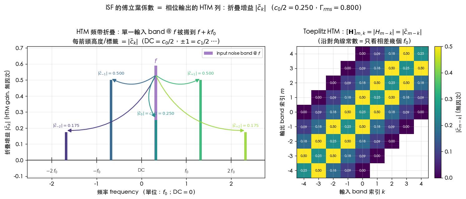
(Figure: simulations/fig_htm_bandfold.py. This is an illustrative teaching figure, not a transistor-level extraction. Left-panel arrow gains $|\tilde c_0|=c_0/2$, $|\tilde c_{\pm1}|=c_1/2$, $|\tilde c_{\pm2}|=c_2/2$ correspond exactly to $H_k^{(\Gamma)}=\tilde c_k$ proven in Step 4; the sum of squared folding gains $\sum_k|\tilde c_k|^2=\Gamma_{rms}^2$ is Step 5's Parseval relation.)

Try it with your own hands — the interactive version below turns the static "single input band, fixed ISF" picture above into a draggable $f_{in}$ with a tunable ISF: drag the slider to sweep the input tone $f_{in}$ from 0 to $3f_0$, and the widget instantly finds the harmonic $k\cdot f_0$ nearest to $f_{in}$ and draws the arrow that folds it down to baseband offset $\Delta f=|f_{in}-k f_0|$; the arrow's height/label is exactly the folding gain $|\tilde c_k|$ ($k=0$ gives $c_0/2$, $k\ge1$ gives $c_k/2$) — a literal, live rendering of the boxed result above and Step 4's $H_k^{(\Gamma)}=\tilde c_k$. Three preset buttons switch the ISF waveform (ideal LC has only $c_1$; asymmetric matches this page's pedagogical ISF figure; square-ish makes the odd harmonics $c_1,c_3$ dominant), and four sliders let you tune $c_0$–$c_3$ freely. The readout cards show the dominant harmonic $k^*$, the baseband offset $\Delta f$, the fold gain $|\tilde c_{k^*}|$, the $\sum|c_k/2|^2$ over the relevant terms (the baseband phase-noise weight), and the integrator $1/(2\pi\Delta f)$ (reading out Step 5's $1/\Delta\omega$ integrator gain too, with $I_0/q_{max}=1$ normalized).

HTM band-folding explorer: drag the input tone, watch it fold to baseband

input tone f_in1.10 f₀ × f₀

ISF preset:

c₀ (DC term)0.50

c₁1.00

c₂0.35

c₃0.18

dominant harmonic k*

k = 1

nearest to f_in

baseband offset Δf

0.100

× f₀ = |f_in − k*·f₀|

fold gain |c̃_k*|

0.500

c1/2

Σ |cₖ/2|² (relevant terms)

0.2500

baseband PN weight

integrator 1/Δω (∝ 1/Δf)

1.59e+0

(units of 1/f₀, unit I₀/q_max)

Model: drag f_in across 0–3 f₀; the widget finds the nearest harmonic k·f₀ (k = 0..3) and draws the folding arrow that lands at baseband offset Δf = |f_in − k f₀|, with gain |c̃_k| = c₀/2 (k=0) or c_k/2 (k≥1) — exactly H_k^(Γ) from Step 4 of this page. A tone parked right on a harmonic (Δf → 0) folds straight to DC with the full gain c_k/2, and the readout integrator 1/(2π Δf) blows up there (the [P1] Eq.16/17 sideband φ_p = I₀ c_k/(2 q_max Δω), shown here with I₀/q_max normalized to 1). Anchor case: pick ideal LC (only c₁ ≠ 0) — only tones near f₀ fold at all; every other harmonic band has zero gain, so Σ|c_k/2|² collapses to the single c₁/2 = 0.5 term. This is a pedagogical toy model (illustrative), not a transistor-level extraction; see ltv_htm Steps 3–5 for the full derivation.

Anchor case (try this): switch to the ideal LC preset ($\Gamma=-\sin\theta$, only $c_1\neq0$). Sweep $f_{in}$ across the whole 0–$3f_0$ window and you will see nonzero folding arrows only while $f_{in}$ passes near $f_0$ — the DC, $2f_0$, and $3f_0$ bands all have zero gain, because the ideal LC's ISF has only a fundamental component. The $\sum|c_k/2|^2$ readout likewise collapses to the single $c_1/2=0.5$ term ($|c_1/2|^2=0.25$). This is direct visual evidence for "an LC oscillator barely folds noise that isn't near an integer multiple of $f_0$"; switch to the asymmetric or square-ish preset and nonzero arrows appear at the DC/higher-harmonic bands as well.

---

Step 4: substitute the oscillator's ISF kernel — $H_k$ is exactly $c_k$

Now we narrow the abstract HTM to [P1]'s phase channel. The phase output's LTV kernel (with respect to noise current) comes from [P1] Eq.(11), written in Step 1's $h(t,\tau)$ form (phase is the cumulative integral of noise, so the kernel carries a unit step):

$$h_\phi(t,\tau)=\frac{\Gamma(\omega_0\tau)}{q_{max}}\,u(t-\tau)\qquad[\text{P1] Eq.(10), p.182}.$$

Substitute the ISF's Fourier series ([P1] Eq.(12), p.183) into $\Gamma$:

$$\Gamma(\omega_0\tau)=\frac{c_0}{2}+\sum_{n=1}^{\infty}c_n\cos(n\omega_0\tau+\theta_n) =\sum_{k=-\infty}^{\infty}\tilde c_k\,e^{jk\omega_0\tau},$$

where the right-hand side rewrites the real-valued cosine series as a complex exponential series ($\tilde c_0=c_0/2$, $\tilde c_{\pm k}=\tfrac12 c_k e^{\pm j\theta_k}$, $k\ge1$; this is the standard real↔complex Fourier conversion, see math_identities).

Core algebra: the phase channel is "ISF-weight, then integrate." First look at the "ISF weighting" — an instantaneous multiplication (we leave the integrator to the next step, since it multiplies every band uniformly by $1/(j2\pi f)$ and does not couple bands). Weight a pure sinusoidal noise $i_n(\tau)=e^{j2\pi f\tau}$ by the ISF:

$$\Gamma(\omega_0\tau)\,e^{j2\pi f\tau} =\sum_{k}\tilde c_k\,e^{jk\omega_0\tau}\,e^{j2\pi f\tau} =\sum_{k}\tilde c_k\,e^{j2\pi (f+kf_0)\tau}.$$

(using $k\omega_0\tau=2\pi(kf_0)\tau$). Comparing against Step 3's $y=\sum_k H_k(f)e^{j2\pi(f+kf_0)t}$, term-by-term matching reads off the harmonic transfer function of the ISF-weighting stage:

$$\boxed{\ H_k^{(\Gamma)}=\tilde c_k\ }\qquad\Longleftrightarrow\qquad H_0^{(\Gamma)}=\frac{c_0}{2},\quad H_{\pm k}^{(\Gamma)}=\tfrac12 c_k\,e^{\pm j\theta_k}\ (k\ge1).$$

• This is half of this page's signature result: the harmonic gain of the ISF-weighting stage's HTM is exactly the ISF's Fourier coefficient. "Input frequency $f$ is shifted to $f+kf_0$ with gain $c_k$" is now a theorem that holds verbatim, not an analogy.
• $H_0=c_0/2$ (the DC band, shifting $f$ right back to itself) — this is exactly the band by which $c_0$ upconverts baseband flicker; $H_{\pm1}\propto c_1$ folds down the band near $\omega_0$ — this exactly matches fourier_series_of_isf Steps 4 and 5.
• Dimension check: $c_k$ is dimensionless, $1/q_{max}$ carries $\text{C}^{-1}$; the ISF channel turns current (A) into a phase rate of change, with the dimension being reconciled to rad by $1/q_{max}$ together with the following integrator (see next step) ✓.

Hands-on verification: $H_k=c_k$ is not an analogy — it's a measurable number

The block below can be run directly (it depends on this site's simulations/common/isf_utils). It tests the claim $H_k=\tilde c_k$ verbatim: separately inject equal-amplitude single-tone noise near $1\omega_0$, $2\omega_0$, $3\omega_0$ (each offset by $\Delta f$), integrate into phase $\phi(t)$, take the FFT of $\phi(t)$, and measure the amplitude of the "sideband down-converted to baseband $\Delta f$." If $H_n\propto c_n$, these sideband ratios must equal the ratios of the ISF's Fourier coefficients $c_1:c_2:c_3$.

import numpy as np
from simulations.common.isf_utils import (
    compute_fourier_coefficients, integrate_phase_from_noise)

f0, qmax = 5e9, 1e-12                 # 5 GHz carrier, q_max = 1 pC
w0 = 2 * np.pi * f0
fs = 8 * f0                           # resolves up to ~3 w0 without aliasing
df = 5e6                              # injected single-tone offset near each harmonic [Hz]
N  = 1 << 21                          # large N -> cleanly resolve the baseband df sideband
t  = np.arange(N) / fs

# same pedagogical ISF as this page's figure / lab_05 (nonzero c0, several nontrivial harmonics):
def gamma(theta):
    return (-np.sin(theta) + 0.35*np.sin(2*theta)
            + 0.18*np.cos(3*theta) + 0.25)

g_traj = gamma(w0 * t)                # Gamma(w0 t), sampled along the trajectory
th = np.linspace(0, 2*np.pi, 4000, True)
_, _, _, c, _ = compute_fourier_coefficients(th, gamma(th), 4)
print(np.round(c[:4], 3))             # -> [0.5  1.    0.35 0.18]  (c0, c1, c2, c3)

I0 = 1e-6
def phi_sideband(n):                  # inject I0 cos((n w0 + df) t), measure phi's sideband at df
    i_n = I0 * np.cos((n*w0 + 2*np.pi*df) * t)
    phi = integrate_phase_from_noise(t, i_n, g_traj, qmax)
    P = np.abs(np.fft.rfft((phi - phi.mean()) * np.hanning(N))) / N
    f = np.fft.rfftfreq(N, 1/fs)
    k = int(np.argmin(np.abs(f - df)))
    return P[k-5:k+6].max()

a1, a2, a3 = (phi_sideband(n) for n in (1, 2, 3))
print(f"a1/a2 = {a1/a2:.3f}   c1/c2 = {c[1]/c[2]:.3f}")  # -> a1/a2 = 2.857   c1/c2 = 2.857
print(f"a1/a3 = {a1/a3:.3f}   c1/c3 = {c[1]/c[3]:.3f}")  # -> a1/a3 = 5.556   c1/c3 = 5.556

The two sets of ratios match digit-for-digit: $\phi$'s response strength to "injection near $n\omega_0$" is proportional to $c_n$, which is the numerical witness to $H_n^{(\Gamma)}=\tilde c_n$ — the HTM's folding gain is the ISF's Fourier coefficient, not an analogy. (This also corresponds to the arrow heights on the left side of the band-folding figure above, $|\tilde c_{\pm1}|=c_1/2$, $|\tilde c_{\pm2}|=c_2/2$.)

---

Step 5: adding back the integrator and $1/q_{max}$ — the complete HTM row of the phase channel

The full phase channel is "ISF weighting $\to$ multiply by $1/q_{max}$ $\to$ integrate" (see the block diagram in white_noise_to_phase_noise). In the frequency domain, the integrator multiplies the "post-shift" frequency $f+kf_0$ by $\dfrac{1}{j2\pi(f+kf_0)}$. But what we care about is phase noise near the carrier: noise falling at $f=-kf_0+\Delta f$ (i.e., "the $k$-th harmonic band offset by $\Delta f$") gets shifted by $H_{k}$ to baseband $\Delta f$ (following Step 3's HTM convention $y=\sum_m H_m\,x(f-mf_0)$, shifting input $-kf_0+\Delta f$ to $\Delta f$ requires $m=k$), and the integrator there multiplies by $\dfrac{1}{j2\pi\Delta f}$. So the gain of the entire chain "noise in the $k$-th band → phase at $\Delta f$ near the carrier" is

$$\frac{1}{q_{max}}\cdot \underbrace{\tilde c_{k}}_{\text{ISF shift}}\cdot\underbrace{\frac{1}{j2\pi\Delta f}}_{\text{integrator}} \;\xrightarrow{\ |\cdot|\ }\; \frac{|c_k|}{2\,q_{max}}\cdot\frac{1}{2\pi\Delta f}\quad(k\ge1).$$

This is exactly [P1] Eq.(16/17), p.183's single-tone sideband result $\phi_p=\dfrac{I_0\,c_k}{2q_{max}\,\Delta\omega}$ ($\Delta\omega=2\pi\Delta f$) — we've re-derived it from the HTM, with every piece (ISF shift $=c_k$, integrator $=1/(j2\pi\Delta f)$, normalization $=1/q_{max}$) cleanly separated out.

Collect this entire row of gains "each input harmonic band → phase output" into a vector (this is the row of the HTM corresponding to the "phase output"):

$$\boxed{\ \mathbf{g}_\phi=\frac{1}{q_{max}}\big[\dots,\ \tilde c_{-2},\ \tilde c_{-1},\ \tfrac{c_0}{2},\ \tilde c_{1},\ \tilde c_{2},\ \dots\big]\ }$$

• The $k$-th component $=\tilde c_k/q_{max}$: maps "the noise band a distance $kf_0$ from the carrier" to phase. The sum of squared magnitudes $\sum_k|\tilde c_k|^2=(c_0/2)^2+\tfrac12\sum_{n\ge1}c_n^2=\Gamma_{rms}^2$ (the DC term contributes as $(c_0/2)^2$, consistent with lab_05's Parseval correction and [P1] Eq.(20)) — this is the HTM version of white_noise_to_phase_noise's use of Parseval to convert $\sum c_n^2$ into $\Gamma_{rms}^2$: the total phase-noise weight = the energy of this conversion vector.
• Dimension check: each component $\tilde c_k/q_{max}$ carries $\text{C}^{-1}$; multiplying by the noise band's charge (A·s/...) and the integrator afterward yields rad ✓.

---

Step 6: conclusion — "the ISF is exactly the conversion vector from each harmonic to the phase output"

Combining Steps 4 and 5, this page's signature theorem holds:

Theorem (ISF = HTM row of the phase output): treat the periodic-time-varying oscillator's phase channel as an LPTV system, indexing input/output by harmonic bands spaced by $f_0$. Then the $k$-th component of the conversion vector $\mathbf{g}_\phi$ mapping "each input harmonic band → phase output" is exactly the (complex) ISF Fourier coefficient divided by $q_{max}$: $[\mathbf{g}_\phi]_k=\tilde c_k/q_{max}$. Equivalently, the ISF's Fourier series $\{c_k\}$ is exactly the content of that row of the phase output in the HTM.

This upgrades three statements that had been treated as "intuition/analogy" into theorems of LTV system theory:

What this site has said (intuition)	Rigorous HTM statement	Correspondence
The oscillator is a "time-varying mixer"	LPTV system, $H(f,t)=\sum_k H_k(f)e^{jk\omega_0 t}$, off-diagonal	Input $f$ → output $f+kf_0$
"Noise near $n\omega_0$ is shifted to the carrier"	$H_{\pm k}^{(\Gamma)}=\tfrac12 c_k e^{\pm j\theta_k}$	Shift gain $=c_k$
"The ISF's Fourier coefficient $c_k$ is the mixer gain"	$[\mathbf{g}_\phi]_k=\tilde c_k/q_{max}$	ISF $=$ HTM row of the phase output
"Total weight $\sum c_n^2=2\Gamma_{rms}^2$"	Conversion-vector energy $\sum_k\vert \tilde c_k\vert ^2=\Gamma_{rms}^2$	Parseval = vector norm

• Relation to [P1] Eq.(13) (within the 5 PDFs): [P1] Eq.(13), p.183 writes phase as "the $c_0$-term integral plus the sum of integrals weighted by each harmonic $c_n\cos(n\omega_0\tau+\theta_n)$." That is exactly the time-domain version of "applying the conversion vector $\mathbf{g}_\phi$ to the noise, then integrating" — the HTM is its frequency-domain counterpart. The two are the same thing in two languages (time-domain series vs. frequency-domain band matrix).
• Relation to PPV/Floquet: derivation_floquet_ppv proves the ISF $=$ the PPV's component at the injection node ($\Gamma/q_{max}=v_1^T\mathbf b$). The HTM is the frequency-domain/system-theory face of "the same ISF"; the PPV is its state-space/differential-geometry face. All three ([P1]'s intuition, PPV, HTM) describe the same object $\Gamma$, just at different levels of abstraction.

---

Comparison table against the three great signals-and-systems objects

Placing this page's LTV objects side by side with the reader's familiar LTI objects completes the map:

Concept	LTI (signals and systems course)	LTV (this page)	Periodic LTV / oscillator
impulse response	$h(t-\tau)$	$h(t,\tau)$	$h(t,\tau)=\frac{\Gamma(\omega_0\tau)}{q_{max}}u(t-\tau)$
output	convolution $\int h(t-\tau)x\,d\tau$	$\int h(t,\tau)x\,d\tau$	[P1] Eq.(11)
transfer function	a single $H(f)$	$H(f,t)$ (Zadeh)	$H(f,t)=\sum_k H_k(f)e^{jk\omega_0 t}$
frequency-domain structure	diagonal (no new frequencies)	general	Toeplitz HTM (shift $kf_0$)
what "transfer function" is	scalar $H(f)$	function $H(f,t)$	matrix $\mathbf H$ (HTM)
phase-channel gain	—	—	conversion vector $\mathbf g_\phi$, $[\mathbf g_\phi]_k=\tilde c_k/q_{max}$

---

Validity and failure conditions

Condition	When it holds	What happens when it fails
System linearity (small perturbation)	Convolution/Zadeh/HTM all hold	Large injection → nonlinearity, harmonic interaction, HTM no longer a single linear map
Periodic steady state (LPTV)	$H(f,t)$ is $T$-periodic in $t$, expandable as $\sum_k H_k$	Startup transient/pulled by injection → not purely periodic, HTM fails
Noise is additive	Conversion vector $\mathbf g_\phi$ acts linearly	Strong multiplicative/cyclostationary effects must first be absorbed into $\Gamma_{eff}=\Gamma\alpha$ (see effective_isf)
Only the phase-output row is taken	$\mathbf g_\phi$ is the ISF	To also track amplitude → need the HTM's "amplitude output row" (corresponds to APF [P4])
Finite band truncation $k$	Low-order $c_k$ dominate, fast numerical convergence	When ISF high-order harmonics are strong, more bands must be retained

---

Correspondence to papers/equations

• This site's main thread (within the 5 PDFs): LTV convolution [P1] Eq.(11), ISF Fourier series [P1] Eq.(12), harmonic-resolved phase response [P1] Eq.(13), p.182–183 (see convolution_derivation, fourier_series_of_isf). This page's HTM is a frequency-domain restatement of Eq.(13).
• Re-derivation of the single-tone sideband via HTM: matches back to [P1] Eq.(16/17), p.183 (Step 5).
• The other face of the rigorous foundation: PPV/Floquet (ISF $=v_1^T\mathbf b$), see derivation_floquet_ppv (external [E2] Demir 2000).
• This page's LTV system framework (Zadeh $H(f,t)$, HTM) is external literature, not among the 5 PDFs: [E5] L. A. Zadeh, "Frequency Analysis of Variable Networks," Proc. IRE 38(3):291–299, Mar. 1950; the HTM is the standard form in LPTV/RF literature. (The formal [E5] Zadeh 1950 citation is recorded in references, DOI 10.1109/JRPROC.1950.231083.)

Key takeaways

• LTI is described by a single $h(t-\tau)$/$H(f)$, diagonal in frequency domain, generating no new frequencies; LTV's kernel becomes $h(t,\tau)$, with output $y=\int h(t,\tau)x\,d\tau$; the oscillator's $h_\phi(t,\tau)=\frac{\Gamma(\omega_0\tau)}{q_{max}}u(t-\tau)$ is exactly one example.
• Zadeh's time-varying transfer function $H(f,t)=\int h(t,t-\sigma)e^{-j2\pi f\sigma}d\sigma$ describes "the instantaneous gain at frequency $f$ right now"; it degenerates to $H(f)$ when time-invariant.
• Periodic LTV (LPTV): $H(f,t)=\sum_k H_k(f)e^{jk\omega_0 t}$; an input frequency $f$ gets shifted to an entire row $f+kf_0$, with gain $H_k$. This set of harmonic gains forms the Toeplitz harmonic transfer matrix (HTM).
• Substituting the ISF kernel → $H_k^{(\Gamma)}=\tilde c_k$ (the ISF's Fourier coefficient); adding back $1/q_{max}$ and the integrator re-derives [P1] Eq.(16/17)'s single-tone sideband.
• Signature theorem: the phase-output conversion vector $[\mathbf g_\phi]_k=\tilde c_k/q_{max}$ — the ISF is exactly the conversion vector from each harmonic band to the phase output (the HTM's phase-output row); its energy $\sum_k|\tilde c_k|^2=\Gamma_{rms}^2$ is Parseval.
• The entire Zadeh/HTM apparatus belongs to external LTV system theory, not among the 5 PDFs ([E5] Zadeh 1950); together with [P1] Eq.(13) and PPV, it is the same ISF in three languages.

Further reading

• The essential difference between LTV and LTI (intuition version): lti_vs_ltv
• The ISF's Fourier coefficients and the mixer picture (the time-domain face of the HTM): fourier_series_of_isf
• Step-by-step derivation of the LTV convolution: convolution_derivation
• The other face of the rigorous foundation (PPV/Floquet/adjoint): derivation_floquet_ppv
• A DSP view of phase noise (frequency shift + integrator): dsp_view_of_phase_noise
• Cyclostationarity and $\Gamma_{eff}$ (the modulation absorbed before the HTM): effective_isf
• Full literature and external citations: references