β: This English translation is in beta — the Traditional-Chinese original is the authoritative version.

Floquet / adjoint / PPV: the rigorous foundation of the ISF

Prerequisites / See also: isf_definition (the intuitive definition of the ISF, "projection onto the tangential direction"), phase_vs_amplitude_noise (geometric picture of phase/amplitude perturbations), lti_vs_ltv (why an oscillator is LTV) | Next: ltv_htm (the HTM face of the same ISF), derivation_leeson (comparison with the empirical model)

[P1] introduces the ISF (Impulse Sensitivity Function) via "physical intuition + impulse simulation": poke the oscillator, see how much the phase permanently shifts, and package the result into a periodic function $\Gamma(\omega_0\tau)$. This route is very approachable and is the main line of this site (see isf_definition). But it leaves one thing unresolved: what exactly, mathematically, is "projection onto the tangential (phase) direction"? Why does that particular direction correspond to "zero restoring force, permanent accumulation"? This page fills in that rigorous mathematical foundation.

Honesty note (read this first): The Floquet theory, monodromy matrix, adjoint method, and PPV (Perturbation Projection Vector) on this page are entirely external literature, not among the five PDFs downloaded for this site. The primary sources are [E2] A. Demir, A. Mehrotra, and J. Roychowdhury, "Phase Noise in Oscillators: A Unifying Theory and Numerical Methods for Characterization," IEEE Trans. Circuits Syst. I, vol. 47, no. 5, pp. 655–674, May 2000, and [E3] F. X. Kärtner, "Analysis of White and $f^{-\alpha}$ Noise in Oscillators," Int. J. Circuit Theory Appl., vol. 18, pp. 485–519, 1990. Volume/issue/page/DOI have been verified online ([E2] DOI 10.1109/81.847872, [E3] DOI 10.1002/cta.4490180505). The notation used on this page ($v_1,B,\xi$, Floquet-exponent conventions) follows the original sources and is presented here as background framework. This page only supplies the mathematical intuition and skeleton for "why the ISF is a rigorous object" — it does not replace the originals.

This page answers three questions:

1. What linear equation governs a perturbation near an oscillator's limit cycle?
2. What is the structure of that equation's solutions (Floquet)? Why must there be a direction with "zero exponent, permanent, undamped"?
3. Projecting an arbitrary perturbation onto that direction, how do we get $\dot\phi=v_1^T(t)B(t)\xi(t)$, and how does that map back onto the ISF's $\Gamma/q_{max}$?

Physical intuition (the punchline first): An autonomous oscillator (one with no external clock, one that determines its own phase) has an intrinsic symmetry — time-translation invariance. Shift the entire solution slightly forward or backward in time, and it's still a valid solution. This direction of "sliding a bit along the trajectory" is the phase direction; since nothing pulls it back to some "correct" instant, a perturbation along this direction stays forever. Floquet theory encodes this as "one Floquet exponent is exactly 0," and the PPV $v_1(t)$ is the weighting vector that converts "an arbitrary kick" into "how far it moved along that direction." The ISF is nothing more than the scalarized version of the PPV for the specific kick "charge injected into a particular node capacitance."

Step 0: writing the oscillator as a state equation

Any oscillator (LC, ring, Colpitts...) can be written as a set of first-order ODEs (state-space form):

$$\dot{\mathbf{x}}(t)=\mathbf{f}\big(\mathbf{x}(t)\big),\qquad \mathbf{x}\in\mathbb{R}^{N}.$$

• $\mathbf{x}$ is the state vector (e.g., $(v_C,\,i_L)$: capacitor voltage, inductor current), $N$ is the state dimension.
• $\mathbf{f}$ is the circuit's nonlinear vector field (device characteristics + KCL/KVL).
• Autonomous: $\mathbf{f}$ has no explicit $t$-dependence — this is precisely the mathematical signature of "the oscillator determines its own frequency and phase."

At steady state there exists a periodic solution $\mathbf{x}_s(t)=\mathbf{x}_s(t+T)$, $T=1/f_0$, tracing a limit cycle in state space.

• Dimension check: $[\dot{\mathbf{x}}]=[\mathbf{x}]/\text{s}$, $[\mathbf{f}]=[\mathbf{x}]/\text{s}$ ✓ (both sides are "rate of change of state").

Injecting noise/perturbation adds a term:

$$\dot{\mathbf{x}}(t)=\mathbf{f}\big(\mathbf{x}(t)\big)+B(t)\,\boldsymbol{\xi}(t).$$

• $\boldsymbol{\xi}(t)$ is the vector of perturbation sources (e.g., various noise currents $i_n$).
• $B(t)$ is the injection/coupling matrix: it specifies which states the perturbation hits, and how strongly. For "current injected into a node capacitance," the corresponding row of $B$ is roughly $1/C_{node}$ (converting current into $\dot v$).
• Dimension check: $[B\boldsymbol\xi]$ must be $[\mathbf{x}]/\text{s}$. If $\xi$ is a current (A) and the corresponding state is a capacitor voltage (V), that row scales as $\sim 1/C$ ($[\text{A}]/[\text{F}]=[\text{A}]\cdot[\text{V/C}]=[\text{V/s}]$) ✓.

Mapping to [P1]'s language: Step 0's $B(t)\boldsymbol\xi(t)$ is exactly the step "noise current through a node capacitance becomes $\dot v$" ([P1] Eq.(9), p.181, the differential form of $\Delta V=\Delta q/C_{node}$).

Step 1: linearizing near the limit cycle → a linear system with periodic coefficients

Under a small perturbation, write $\mathbf{x}(t)=\mathbf{x}_s(t)+\Delta\mathbf{x}(t)$ and Taylor-expand $\mathbf{f}$ to first order:

$$\dot{\mathbf{x}}_s+\dot{\Delta\mathbf{x}}=\mathbf{f}(\mathbf{x}_s)+\underbrace{\frac{\partial\mathbf{f}}{\partial\mathbf{x}}\bigg|_{\mathbf{x}_s(t)}}_{\equiv\,A(t)}\Delta\mathbf{x}+B(t)\boldsymbol\xi(t)+O(\Delta\mathbf{x}^2).$$

Since $\dot{\mathbf{x}}_s=\mathbf{f}(\mathbf{x}_s)$ (the steady state itself satisfies the unperturbed equation), the two sides cancel, leaving the linear equation for the perturbation:

$$\dot{\Delta\mathbf{x}}(t)=A(t)\,\Delta\mathbf{x}(t)+B(t)\,\boldsymbol\xi(t),\qquad A(t)\equiv\frac{\partial\mathbf{f}}{\partial\mathbf{x}}\bigg|_{\mathbf{x}_s(t)}.$$

• Key observation: $A(t)=A(t+T)$ is a matrix with periodic coefficients (because it's evaluated on the periodic trajectory $\mathbf{x}_s(t)$). This is exactly why oscillator perturbations are LTV (linear time-varying) rather than LTI — the "system matrix" varies periodically in time, matching the LTV nature that [P1] repeatedly emphasizes (see lti_vs_ltv).
• Math used: Jacobian linearization; dropping $O(\Delta\mathbf{x}^2)$ is the "small perturbation/small noise" assumption, consistent with [P1]'s small-signal assumption.
• Dimension check: $A$ has units $1/\text{s}$ ($\partial\dot{\mathbf x}/\partial\mathbf x$), and $A\,\Delta\mathbf x$ is $[\mathbf x]/\text{s}$ ✓.

The homogeneous part (turning off $\boldsymbol\xi$) is

$$\dot{\Delta\mathbf{x}}=A(t)\,\Delta\mathbf{x},\qquad A(t+T)=A(t).$$

This is precisely the object studied by Floquet theory: a linear ODE with periodic coefficients.

Step 2: Floquet theory — solution structure and the monodromy matrix

For the linear system $\dot{\Delta\mathbf x}=A(t)\Delta\mathbf x$, define the state transition matrix $\Phi(t,t_0)$: it maps a perturbation at time $t_0$ to time $t$, $\Delta\mathbf x(t)=\Phi(t,t_0)\Delta\mathbf x(t_0)$, with $\Phi(t_0,t_0)=I$.

Advancing it over exactly one period gives the monodromy matrix:

$$M\equiv\Phi(t_0+T,\,t_0).$$

• Physical meaning: $M$ answers "what does a perturbation become after one full cycle?" Its eigenvalues $\mu_i$ are called Floquet multipliers, describing the amplification/attenuation factor per cycle for each perturbation direction.
• Dimension check: $\Phi$ and $M$ are both dimensionless linear maps (state to state) ✓.

Floquet's theorem states that homogeneous solutions can be written as

$$\Delta\mathbf{x}(t)=\sum_{i=1}^{N} c_i\,\mathbf{u}_i(t)\,e^{\lambda_i t},\qquad \mathbf{u}_i(t)=\mathbf{u}_i(t+T),$$

where $\mathbf{u}_i(t)$ is the periodic Floquet eigenvector and $\lambda_i$ are the Floquet exponents, related to the multipliers by

$$\mu_i=e^{\lambda_i T}\quad\Longleftrightarrow\quad \lambda_i=\frac{1}{T}\ln\mu_i.$$

• How to read $\lambda_i$: $\mathrm{Re}\,\lambda_i<0$ → the perturbation along that direction decays (stable, e.g., the amplitude direction); $\mathrm{Re}\,\lambda_i=0$ → neutral, undamped (the phase direction); $\mathrm{Re}\,\lambda_i>0$ → diverges (should not occur for a stable limit cycle).
• Dimension check: $[\lambda_i]=1/\text{s}$, $[\lambda_i T]$ dimensionless (the exponent must be dimensionless) ✓.

Step 3: why there must be a $\lambda=0$ direction (the phase direction)

This is the pivot of the whole theory, and it can be proven by hand. Differentiate the steady-state solution with respect to time: differentiate both sides of $\dot{\mathbf x}_s=\mathbf f(\mathbf x_s)$ once more with respect to $t$ (chain rule):

$$\frac{d}{dt}\dot{\mathbf x}_s=\frac{\partial\mathbf f}{\partial\mathbf x}\bigg|_{\mathbf x_s}\dot{\mathbf x}_s \quad\Longrightarrow\quad \frac{d}{dt}\big(\dot{\mathbf x}_s\big)=A(t)\,\dot{\mathbf x}_s.$$

In other words, $\dot{\mathbf x}_s(t)$ is itself a solution of the homogeneous perturbation equation $\dot{\Delta\mathbf x}=A(t)\Delta\mathbf x$! And $\dot{\mathbf x}_s(t)=\dot{\mathbf x}_s(t+T)$ is periodic — it carries no exponential growth/decay factor at all, i.e., $\lambda=0$ in $e^{\lambda t}$.

• Conclusion: the Floquet exponent corresponding to the tangent vector $\dot{\mathbf x}_s(t)$ of the limit cycle is exactly $\lambda_1=0$. Denote it the first principal vector:

$$\mathbf{u}_1(t)\propto\dot{\mathbf x}_s(t),\qquad \lambda_1=0.$$

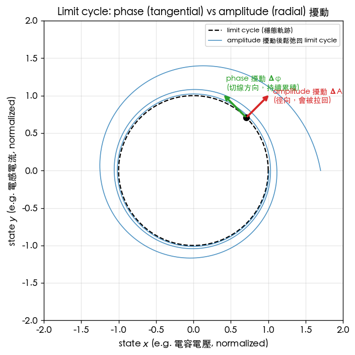
How to read this figure: the tangential arrow along the limit cycle in the figure is exactly the $\mathbf u_1(t)\propto\dot{\mathbf x}_s(t)$ just proven in this step — it corresponds to $\lambda_1=0$, so a perturbation along this direction neither grows nor decays, and accumulates permanently as phase; the radial arrow (amplitude direction) corresponds to $\mathrm{Re}\,\lambda_{i\ge2}<0$, where the perturbation is pulled back to the limit cycle by a restoring force. This is exactly the rigorous Floquet version of the geometric picture in phase_vs_amplitude_noise (same figure limit_cycle_phase_amplitude.png, lab_01 fig_limit_cycle, pedagogical toy model, 2-D state illustration).

• Physical meaning: $\dot{\mathbf x}_s$ is the direction of "moving along the trajectory." Moving along this direction = shifting in time = changing phase. $\lambda_1=0$ mathematically guarantees that "phase perturbation neither amplifies nor decays, and is retained forever" — this is exactly the rigorous basis for [P1]'s expression of "a phase step never disappears" via the unit step $u(t-\tau)$ ([P1] Eq.(10), p.182), and for the statement in Step 2 of isf_definition that "the tangential direction = neutral direction, no restoring force."
• Other directions: the remaining $\lambda_2,\dots$ (amplitude and faster-decaying modes) have $\mathrm{Re}\,\lambda_i<0$, so the perturbation is pulled back to the limit cycle — this is the rigorous version of "amplitude perturbation decays" ([P4] Fig. 5, p.2126, the amplitude decay function, see phase_vs_amplitude_noise).

This step is the entire secret behind the ISF's "projection onto the tangential direction": this site's isf_definition dots the perturbation with $\partial\mathbf z/\partial\theta$ by hand; and $\partial\mathbf z/\partial\theta\propto\dot{\mathbf x}_s$ is precisely the Floquet principal vector with $\lambda_1=0$. Intuition and rigor line up perfectly here.

Step 4: the adjoint system and the "left eigenvector" $v_1(t)$

Here's the issue: $\mathbf{u}_1(t)$ tells us what the phase direction looks like, but to project an arbitrary kick $B(t)\boldsymbol\xi(t)$ onto the phase direction, we need its dual — a left vector capable of "extracting the phase component." This is where the adjoint system comes in.

Define the adjoint equation of the original system:

$$\dot{\mathbf{p}}(t)=-A^{T}(t)\,\mathbf{p}(t).$$

• Why $-A^T$: consider the inner product $\langle\mathbf p,\Delta\mathbf x\rangle=\mathbf p^T\Delta\mathbf x$, and apply the product rule:

$$\frac{d}{dt}\big(\mathbf p^T\Delta\mathbf x\big)=\dot{\mathbf p}^T\Delta\mathbf x+\mathbf p^T\dot{\Delta\mathbf x} =(-A^T\mathbf p)^T\Delta\mathbf x+\mathbf p^T(A\,\Delta\mathbf x) =-\mathbf p^TA\,\Delta\mathbf x+\mathbf p^TA\,\Delta\mathbf x=0.$$

So choosing $\dot{\mathbf p}=-A^T\mathbf p$ makes the inner product $\mathbf p^T\Delta\mathbf x$ conserved — exactly the property we need: "the projection is not corrupted by the system's evolution."

• Dimension check: $[-A^T\mathbf p]=[\mathbf p]/\text{s}$ ✓ (consistent with $\dot{\mathbf p}$).

The adjoint system also has Floquet structure, and the periodic solution corresponding to $\lambda=0$ is denoted $v_1(t)$ — it is the dual (left Floquet vector) of the original system's $\mathbf u_1(t)$. $v_1(t)$ is the PPV (Perturbation Projection Vector). The standard normalization is "the PPV is aligned with the phase direction with unit scale":

$$v_1^{T}(t)\,\dot{\mathbf x}_s(t)=1\qquad\text{(for all }t\text{; normalization convention)}.$$

• Intuition: $\mathbf u_1\propto\dot{\mathbf x}_s$ is "the arrow of the phase direction"; $v_1$ is "the ruler that measures the component along that arrow." The two are calibrated by the equation above so that "moving one unit of time along the trajectory = phase advances by one unit."
• Practical value of the adjoint: solving the adjoint system's periodic solution once gives you the entire $v_1(t)$ in one shot (i.e., the entire ISF); no need to brute-force "fire an impulse at one phase at a time" as in lab_04. The PSS + Pnoise engines inside commercial RF simulators internally use exactly this kind of adjoint/Floquet flow.
• Note (background): the normalization convention for $v_1(t)$ ($v_1^T\dot{\mathbf x}_s=1$) and the $\lambda$ notation follow [E2] Demir 2000 (pp.655–674, DOI 10.1109/81.847872); the citation has been verified, but the internal notation belongs to an external framework.

Step 5: projection → proving $\dot\phi=v_1^T(t)B(t)\boldsymbol\xi(t)$

Now apply the "ruler" from Step 4 to the perturbed equation. Demir et al. prove that, near the limit cycle, the state can be written as "a phase shift along the trajectory + a decaying orbital deviation":

$$\mathbf{x}(t)=\mathbf{x}_s\big(t+\alpha(t)\big)+\mathbf{y}(t),$$

where $\alpha(t)$ is the phase shift in the time domain (units s), and $\mathbf y(t)$ is the decaying orbital-deviation component (lying in the subspace with $\mathrm{Re}\,\lambda<0$). Substitute this back into $\dot{\mathbf x}=\mathbf f(\mathbf x)+B\boldsymbol\xi$, and use $v_1$ to project out the decaying $\mathbf y$ (because $v_1^T$ is "orthogonal" to those directions — this is the biorthogonality of the left/right Floquet vectors). Only the phase component survives, giving the first-order phase equation:

$$\dot{\alpha}(t)=v_1^{T}\big(t+\alpha(t)\big)\,B(t)\,\boldsymbol\xi(t)\;\approx\;v_1^{T}(t)\,B(t)\,\boldsymbol\xi(t).$$

Converting the time-domain phase $\alpha$ into the radian phase $\phi=\omega_0\alpha$ (or directly defining $\phi$ as the dimensionless phase) gives this page's headline result:

$$\boxed{\ \dot{\phi}(t)=v_1^{T}(t)\,B(t)\,\boldsymbol\xi(t)\ }$$

• Term-by-term meaning: $\boldsymbol\xi(t)$ is the raw perturbation (noise current); $B(t)$ injects it into state space (via the node capacitance); $v_1^T(t)$ projects the result onto the phase direction, extracting "how much phase-change rate this particular kick contributes."
• Why $\dot\phi$ (rate) rather than $\phi$: because the phase is the neutral direction ($\lambda_1=0$), every instantaneous kick is accumulated into the phase "verbatim" — so the perturbation directly gives $\dot\phi$; to get $\phi$ you must integrate over time. This is exactly the same as the integral form of [P1] Eq.(11) (convolution_derivation):

$$\phi(t)=\int_{-\infty}^{t}v_1^{T}(\tau)\,B(\tau)\,\boldsymbol\xi(\tau)\,d\tau.$$

• Dimension check: $\dot\phi$ is in rad/s. On the right, $v_1^TB\boldsymbol\xi$: taking noise as a current (A), the corresponding row of $B$ scales as $\sim1/C$ (V/C via A becomes V/s... details depend on normalization), and the overall combination is tuned to rad/s. The exact dimensional bookkeeping depends on the normalization of $v_1$ (whether it absorbs $1/q_{max}$) (following [E2]'s convention) — see the next step for the mapping.

Step 6: mapping back to the ISF — $\Gamma/q_{max}$ is the scalarized PPV

Narrow Step 5 down to [P1]'s specific scenario: a single noise current $i_n(t)$ injected into a single node capacitance $C_{node}$. In that case:

• $\boldsymbol\xi(t)\to i_n(t)$ (scalar).
• $B(t)\to \mathbf b$ (a constant vector, nonzero only in the entry corresponding to "the capacitor state at the injection node," with value $\sim 1/C_{node}$, converting current into $\dot v$).
• $v_1^T(t)\,\mathbf b$ is a scalar periodic function — it is exactly $\Gamma(\omega_0 t)/q_{max}$.

Therefore

$$\dot\phi(t)=\big[v_1^{T}(t)\,\mathbf b\big]\,i_n(t)\;\equiv\;\frac{\Gamma(\omega_0 t)}{q_{max}}\,i_n(t) \quad\Longrightarrow\quad \phi(t)=\frac{1}{q_{max}}\int_{-\infty}^{t}\Gamma(\omega_0\tau)\,i_n(\tau)\,d\tau.$$

The right-hand form is exactly [P1] Eq.(11), p.182. Comparing the two gives the rigorous correspondence:

$$\boxed{\ \frac{\Gamma(\omega_0\tau)}{q_{max}}=v_1^{T}(\tau)\,\mathbf b=\big(\text{the PPV's component at the injection node}\big)\ }$$

Equivalently, pulling the $q_{max}$ normalization out explicitly, the ISF is "the PPV's component at that node, scaled by $q_{max}$" (matching the authors' convention 10.2: ISF $=q_{max}\cdot$(PPV's component at the injection node)):

$$\Gamma(\omega_0\tau)=q_{max}\cdot\big(\text{the component of }v_1(\tau)\text{ on the capacitor state at the injection node}\big).$$

• Why $\Gamma$ is dimensionless while the PPV has units: the PPV $v_1$ carries units (depending on the physical quantity of the state), but multiplying by $q_{max}=C_{node}V_{max}$ (C) cancels them exactly, turning it into a dimensionless "shape function" — this is the deep reason [P1] normalizes with $q_{max}$ (see Step 3 of isf_definition).
• Why $\Gamma$ has period $2\pi$: $v_1(t)$ is a periodic Floquet vector (period $T$); substituting $\omega_0\tau$ turns the period into $2\pi$ ✓.
• Why "each node/each noise source has its own ISF": because each injection point corresponds to a different $\mathbf b$, projecting out a different scalar $v_1^T\mathbf b$ ✓. This upgrades the property stated in isf_definition from "intuition" to "a choice of column of $B$."

Three-language comparison table

The same thing, at three levels of abstraction:

Concept	[P1] intuitive language (main line of this site)	Floquet/PPV rigorous language (this page, external literature)	Correspondence
Phase direction	tangent to the limit cycle, $\partial\mathbf z/\partial\theta$	Floquet principal vector with $\lambda_1=0$, $\mathbf u_1\propto\dot{\mathbf x}_s$	same direction
"Phase does not decay"	no restoring force on phase, unit step $u(t-\tau)$	Floquet exponent $\lambda_1=0$ (neutral)	$\lambda_1=0\Leftrightarrow$ permanently retained
Projection weight	"conversion ratio" $\Gamma/q_{max}$	node component of PPV $v_1(t)$	$\Gamma/q_{max}=v_1^T\mathbf b$
Phase response	$\phi=\tfrac{1}{q_{max}}\int\Gamma\,i_n\,d\tau$	$\dot\phi=v_1^TB\boldsymbol\xi$ (integrated)	same equation
Extraction method	fire impulses phase by phase (lab_04 brute force)	solve the adjoint periodic solution once, get the whole curve	adjoint is far more efficient
Amplitude decay	amplitude restoring	subspace with $\mathrm{Re}\,\lambda_{i\ge2}<0$	rigorizes "amplitude is pulled back"

Conditions for validity and failure

Condition	When it holds	What happens when it fails
A stable limit cycle exists	Floquet structure holds, $\lambda_1=0$ is the unique neutral direction	with multiple limit cycles/chaos, PPV is non-unique or does not exist
Small perturbation (linearization valid)	$\dot\phi=v_1^TB\boldsymbol\xi$ holds to first order	large injection → must keep the nonlinear phase equation in $\alpha$ (Demir's full expression)
Perturbation is additive, $B\boldsymbol\xi$	projection is clean, $\Gamma_{eff}$ can absorb cyclostationarity (see effective_isf)	strongly multiplicative/state-dependent noise needs a more complete model
Single-node current injection	scalarization $\Gamma/q_{max}=v_1^T\mathbf b$ holds	multi-node/distributed injection must keep the vector form $v_1^TB$

Which papers/equations this maps to

• Main line of this site (within the five PDFs): projection onto the tangential direction, $\Gamma$ dimensionless/periodic, $\phi=\tfrac{1}{q_{max}}\int\Gamma\,i_n\,d\tau$ — [P1] Eqs.(10),(11), p.182 (see isf_definition, convolution_derivation).
• Cyclostationary interface: replacing $\Gamma\to\Gamma_{eff}=\Gamma\alpha$ is compatible with this page's $v_1$-projection framework — [P1] Eqs.(25)–(27), p.186 (see effective_isf).
• All rigorous machinery on this page is external literature, not within the five PDFs: [E2] Demir–Mehrotra–Roychowdhury 2000 (PPV, $\dot\phi=v_1^TB\boldsymbol\xi$), [E3] Kärtner 1990 (analysis of white/$f^{-\alpha}$ perturbations). Formal citation volume/page/DOI have been verified; see references ([E2], [E3]).

Numerical verification: computing the monodromy matrix and PPV by hand

The preceding six steps are all theorems and prose. An old engineer's habit is: don't trust that you truly understand a theorem until it becomes numbers. In this section we take a van der Pol oscillator ($\mu=0.2$, near-harmonic, unit frequency — the same toy as lab_15) and compute every mathematical object on this page as a number, one by one: the limit cycle, $T$, monodromy $M$, Floquet multipliers, adjoint periodic solution $v_1(t)$, and PPV→ISF — then overlay the ISF from the adjoint method on top of the brute-force "fire an impulse at each phase" method (lab_15's approach) in a single figure. Full script: simulations/lab_25_floquet_numeric.py.

Honesty note: this is a pedagogical toy model (not transistor-level); everything uses normalized (dimensionless) units — the time unit is "the second in which the near-harmonic-limit angular frequency $=1$ rad/s," and states $x,y$ are dimensionless. Below, wherever s and rad/s are written, they refer to this normalized unit system. The Floquet/adjoint algorithm itself follows the framework of [E2] Demir 2000 (external literature, not among the five PDFs on this site).

Model and Jacobian (write it once, shared by the next four steps)

The van der Pol equation $\ddot x-\mu(1-x^2)\dot x+x=0$ written in the state form of Step 0:

$$\dot{\mathbf x}=\mathbf f(\mathbf x)=\begin{pmatrix}y\\ \mu(1-x^2)\,y-x\end{pmatrix},\qquad \mathbf x=(x,y),\ \ \mu=0.2 .$$

The Jacobian needed for Step 1, differentiating term by term ($f_2=\mu(1-x^2)y-x$): $\partial f_2/\partial x=-2\mu xy-1$, $\partial f_2/\partial y=\mu(1-x^2)$, so

$$A(t)=\frac{\partial\mathbf f}{\partial\mathbf x}\bigg|_{\mathbf x_s(t)} =\begin{pmatrix}0 & 1\\ -2\mu x_s y_s-1 & \mu(1-x_s^2)\end{pmatrix}, \qquad A(t+T)=A(t).$$

• Dimension check: under normalization, $[x]=[y]=$ dimensionless, $[t]=$ s, so $[A]=1/\text{s}$ ✓ (the general conclusion of Step 1).
• Reason for choosing $\mu=0.2$: small enough → the waveform is nearly sinusoidal, so the ISF should be close to $-\sin$ (checkable against intuition); yet nonzero → the Floquet structure is non-degenerate ($\vert\mu_2\vert$ clearly less than 1).

Numerical step 1: finding the limit cycle and period $T$

Method: starting from $(2,0)$, integrate with RK4 (step size $10^{-3}$ s) for 300 s — the transient decays as $e^{-\mu t}$, and $\mu t=60$ already reaches machine precision; then take the Poincaré section "$x=0$, $y>0$ (rising zero-crossing of $x$)," and use a Newton step $\Delta t=-x/\dot x=-x/y$ to correct the crossing point to $\vert x\vert<10^{-13}$; average over 5 consecutive returns to the section to get $T$.

import numpy as np
from simulations.lab_25_floquet_numeric import find_limit_cycle, monodromy

s0, T = find_limit_cycle()            # step 1: settle + Poincare section + Newton
print(round(T, 4))                    # -> 6.2989
print(round(2 * np.pi / T, 4))        # -> 0.9975

M, states, hf = monodromy(s0, T)      # step 2: dPhi/dt = A(t)Phi integrated over one cycle
mults = np.sort(np.linalg.eigvals(M).real)[::-1]
print(round(float(mults[0]), 6), round(float(mults[1]), 4))  # -> 1.0 0.2828
print(round(float(np.log(mults[1]) / T), 4))                 # -> -0.2005
print(round(float(np.linalg.det(M)), 6))                     # -> 0.282827
tr = 0.2 * (1 - states[:, 0] ** 2)    # tr A = mu(1 - x^2)
print(round(float(np.exp(np.trapezoid(tr, dx=hf))), 6))      # -> 0.282827

Result and cross-check: $T=6.2989$ s, $\omega_0=2\pi/T=0.9975$ rad/s. The Lindstedt–Poincaré perturbation expansion gives the standard van der Pol result $T=2\pi\,(1+\mu^2/16+O(\mu^4))$ (external literature, not among the five PDFs on this site: A. H. Nayfeh, Perturbation Methods, Wiley, New York, 1973): substituting $\mu=0.2$ gives $2\pi\times1.0025=6.2989$ s — matching the numerical result to four decimal places; equivalently $\omega_0\approx1-\mu^2/16=0.9975$ ✓. Amplitude $A=\max\vert x_s\vert=2.0004$ (the well-known result $A\to2$ in the harmonic limit).

• Dimension check: $[T]=$ s, $[\omega_0]=$ rad/s ✓; rad is a dimensionless bookkeeping unit.

Numerical step 2: fundamental matrix over one cycle → monodromy $M$ and multipliers

Method: turn Step 2's definition directly into a numerical problem — integrate "state + fundamental matrix" simultaneously along the cycle just found:

$$\frac{d\Phi}{dt}=A(t)\,\Phi,\qquad \Phi(0)=I_2,\qquad M=\Phi(T),$$

RK4, 12000 steps per period ($A(t)$ is evaluated directly from the current $\mathbf x_s$ at each RK4 stage's Jacobian; no analytic form of $A(t)$ is needed).

Result (printed by the same code block above):

$$\mu_1=1.000000,\qquad \mu_2=0.2828,$$ $$\lambda_1=\frac{\ln\mu_1}{T}=1.5\times10^{-13}\ \text{1/s}\approx0,\qquad \lambda_2=\frac{\ln\mu_2}{T}=-0.2005\ \text{1/s}.$$

Three things worth reading twice:

1. $\mu_1=1$ is not something we put in — it's something that came out. The program was never told at any point that "there is a phase direction"; the deviation of $\mu_1$ from 1 ($\sim10^{-13}$) is simultaneously numerical evidence for Step 3's theorem (tangent direction $\Rightarrow\lambda_1=0$) and a self-diagnostic that "the cycle was found accurately enough, $T$ was measured accurately enough" — if settling is insufficient or $T$ is wrong, $\mu_1$ immediately deviates from 1.
2. $\lambda_2\approx-\mu$ has an analytic counterpart. Using standard averaging (Krylov–Bogoliubov; same Nayfeh 1973, external literature): the slow-amplitude equation $\dot a=g(a)=\tfrac{\mu}{2}a\,(1-a^2/4)$, linearized at $a=2$: $g'(a)=\tfrac{\mu}{2}(1-3a^2/4)$, $g'(2)=\tfrac{\mu}{2}(1-3)=-\mu$. So the first-order prediction is $\lambda_2=-\mu=-0.2$, versus the numerical $-0.2005$ (0.25% difference, an $O(\mu^3)$ correction) ✓. The amplitude-perturbation time constant $\tau_{amp}=1/\vert\lambda_2\vert=4.99$ s $\approx1/\mu$ — this is exactly the Floquet-rigorous version, on this toy, of the amplitude decay function $d=e^{-t/\tau_0}$ in [P4] Fig. 5, p.2126 (LC oscillator $\tau_0=2Q/\omega_0$).
3. Abel–Liouville cross-check. The determinant identity $\det M=\exp\!\big(\int_0^T\operatorname{tr}A\,dt\big)$, with $\operatorname{tr}A=\mu(1-x_s^2)$: left side $\mu_1\mu_2=0.282827$, right side — numerically integrating along the cycle and exponentiating — $=0.282827$ — matching to six decimal places. Two completely independent computational paths (eigenvalues vs. the integral of the trace) agree exactly, confirming the integrator hasn't lost anything.

• Dimension check: $\Phi,M,\mu_i$ are dimensionless (state-to-state maps) ✓; $[\lambda_i]=1/\text{s}$, and $\lambda_iT$ must be dimensionless to sit inside the exponent ✓.

Numerical step 3: integrating the adjoint backward → the periodic left vector $v_1(t)$

Why integrate "backward": first turn Step 4's conservation law into a map. For any initial perturbation $\Delta\mathbf x(0)$, $\mathbf p(T)^T\Delta\mathbf x(T)=\mathbf p(0)^T\Delta\mathbf x(0)$ and $\Delta\mathbf x(T)=M\Delta\mathbf x(0)$, so $M^T\mathbf p(T)=\mathbf p(0)$ — the adjoint's "one-cycle map" is $M^{-T}$, whose eigenvalues are $1/\mu_i$: namely $1$ and $1/0.2828=3.54$. Integrating forward, that 3.54 mode amplifies numerical impurities by 3.54× per cycle, quickly swamping $v_1$; integrating backward, it decays by a factor of 0.2828 per cycle, so the integration automatically "self-cleans" and converges to the periodic solution $v_1(t)$ — this is exactly [E2] Demir 2000's backward-adjoint numerical procedure (external literature). We start from the eigenvalue-$1$ left eigenvector of $M^T$ and integrate backward along the cycle:

$$\dot{\mathbf p}=-A^T(t)\,\mathbf p\quad(\text{integrated from }t=T\text{ back to }t=0).$$

import numpy as np
from simulations.common.isf_utils import gamma_rms
from simulations.lab_25_floquet_numeric import ppv_pipeline

res = ppv_pipeline()                       # steps 1-3 done in one call
print("{:.1e}".format(res["const_err"]))   # -> 2.2e-14
print("{:.1e}".format(res["per_err"]))     # -> 9.5e-13

theta = res["theta"]
g = res["omega0"] * res["v1"][:, 1]        # step 4: Gamma/qmax = w0 * v1_y
print(round(float(np.max(np.abs(g))), 4))  # -> 0.5011
print(round(res["qmax_toy"], 4))           # -> 2.0442
print(round(float(gamma_rms(theta, res["qmax_toy"] * g)), 4))   # -> 0.7258
gn = g / np.max(np.abs(g))
print(round(float(np.sqrt(np.mean((gn + np.sin(theta)) ** 2))), 4))  # -> 0.0555

Two machine-precision-level checks:

• Periodicity: $\Vert\mathbf p(0)-\mathbf p(T)\Vert/\Vert\mathbf p(T)\Vert=9.5\times10^{-13}$ — integrating backward over one cycle does indeed return to itself (the left Floquet vector, $\lambda=0$).

• Constant normalization (the inner-product conservation theorem of Step 4): $\mathbf p(t)^T\dot{\mathbf x}_s(t)$'s maximum relative deviation over the full cycle $=2.2\times10^{-14}$. This inner product should not move by even a constant, theoretically; numerically only round-off error remains. Dividing by this constant completes the normalization $v_1^T(t)\,\dot{\mathbf x}_s(t)=1$ (for all $t$).

• Dimension check: the normalization condition $v_1^T\dot{\mathbf x}_s=1$ (dimensionless) gives $[v_1]=\text{s}/[\mathbf x]$; hence the time-domain phase $\Delta\alpha=v_1^T\Delta\mathbf x$ obtained from a kick $\Delta\mathbf x$ has units of s ✓ (the units of $\alpha(t)$ from Step 5).

Numerical step 4: the components of $v_1$ are the ISF — head-to-head overlay

Step 6 says $\Gamma(\omega_0\tau)/q_{max}=v_1^T\mathbf b$. For this toy we fire the impulse along the $y$-axis (exactly the same kick as lab_15's impulse_dy, $\mathbf b=\hat{\mathbf e}_y$), so

$$\frac{\Gamma(\theta)}{q_{max}}=\omega_0\,v_{1,y}(\theta),\qquad \theta=\omega_0 t\ (\text{measured from the rising zero-crossing of }x).$$

• That $\omega_0$ is a unit conversion, not new physics: $v_1$ gives "how many seconds per unit $\Delta q$" ($\Delta\alpha$, s); multiplying by $\omega_0$ converts it to "how many radians" ($\Delta\phi=\omega_0\Delta\alpha$). This is exactly the same factor this site repeatedly emphasizes in [P2] Eq.(8), p.792 ($\sigma_{\Delta\phi}=\kappa\sqrt{\Delta t}$, phase jitter) and Eq.(12), p.793 (the $\kappa$ expression does not contain $\omega_0$) — "time-domain vs. radian-domain bookkeeping" — and it must be made explicit each time which domain you're working in and when to multiply by $\omega_0$.
• Dimension check: $[\omega_0 v_{1,y}]=(\text{rad/s})\times(\text{s}/[\Delta q])=\text{rad}/[\Delta q]$ ✓ — exactly the units of $\Gamma/q_{max}$ in [P1] Eq.(10), p.182 (phase per unit charge).

Analytic comparison in the harmonic limit ($\mu\to0$, what it should look like): pure harmonic $x=A\sin\theta$, $y=\dot x=\omega_0A\cos\theta$, and the phase can be written $\theta=\operatorname{atan2}(u,v)$, $u=\omega_0x$, $v=y$. Using $\partial\,\mathrm{atan2}/\partial v=-u/(u^2+v^2)$ and $\partial\,\mathrm{atan2}/\partial u=+v/(u^2+v^2)$, with $u^2+v^2=\omega_0^2A^2$:

$$\frac{\Gamma_y(\theta)}{q_{max}}=\frac{\partial\theta}{\partial y} =\frac{-\omega_0A\sin\theta}{\omega_0^2A^2}=-\frac{\sin\theta}{\omega_0A}, \qquad \frac{\Gamma_x(\theta)}{q_{max}}=\frac{\partial\theta}{\partial x} =\omega_0\cdot\frac{\omega_0A\cos\theta}{\omega_0^2A^2}=+\frac{\cos\theta}{A}.$$

Predicted peak $1/(\omega_0A)=1/(0.9975\times2.0004)=0.5011$ — the numerical peak is exactly $0.5011$ ✓.

import numpy as np
from simulations.lab_15_nonlinear_isf import extract_vdp_isf
from simulations.lab_25_floquet_numeric import ppv_isf, extract_isf_impulse_axis

theta, g_ppv, res = ppv_isf()              # adjoint solved once
th15, isf15, T15 = extract_vdp_isf(0.2)    # lab_15 brute force: 36 phases, impulses
rms = np.sqrt(np.mean((np.interp(th15, theta, g_ppv) - isf15) ** 2))
print(round(float(rms), 4))                # -> 0.0016

g_ppv_x = res["omega0"] * res["v1"][:, 0]  # x-component of the same v1
thx, isfx = extract_isf_impulse_axis(res["s0"], res["T"], axis=0)
rms_x = np.sqrt(np.mean((np.interp(thx, theta, g_ppv_x) - isfx) ** 2))
print(round(float(rms_x), 4))              # -> 0.0023

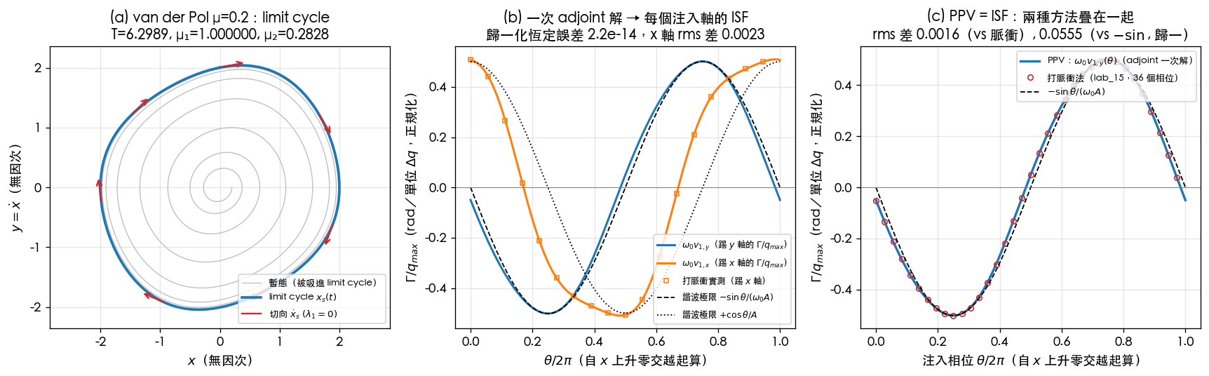
How to read this figure (script: simulations/lab_25_floquet_numeric.py, figure floquet_ppv_numeric.png):

• (a): the gray line is the transient (absorbed into the limit cycle as $e^{\lambda_2 t}$ — a visualization of $\mathrm{Re}\,\lambda_2<0$); the blue circle is $\mathbf x_s(t)$; the red arrow is the tangent $\dot{\mathbf x}_s$, i.e., the Floquet principal vector $\mathbf u_1$ with $\lambda_1=0$.
• (b): a single adjoint solve gives the whole $v_1(t)$, and its two components are simultaneously the ISFs for the two injection axes — the blue line (kicking $y$) hugs $-\sin\theta/(\omega_0A)$; the orange line (kicking $x$) shows a visible deviation from the harmonic limit $+\cos\theta/A$ (dotted line). This deviation is genuine physics (waveform distortion at $\mu=0.2$), not numerical error — the evidence: the orange squares are from a separately performed, independent impulse sweep (kicking the $x$-axis, 18 phases), differing from the orange line by an rms of only $0.0023$. Step 4's claim, "solve the adjoint once and get the ISF for every injection point," becomes a computed fact here: the $x$-axis ISF was obtained without re-solving the adjoint — just reading off a different component of the same $v_1$.
• (c): the headline overlay. Blue line = $\omega_0v_{1,y}$ (adjoint method); red circles = lab_15's impulse-firing method (36 phases, $\Delta q=0.02$); black dashed line = $-\sin\theta/(\omega_0A)$. The raw rms difference between PPV and impulse is $=0.0016$ (0.3% of the peak); after normalization, the rms difference from $-\sin\theta$ is $=0.0555$ — the latter is 30× larger than the former, showing that the "deviation from $-\sin$" part is genuine $O(\mu)$ waveform-distortion physics (both methods measure it consistently), not error.

Tying the toy back to the site's canonical numbers: taking the toy's $q_{max}$ as the maximum swing of the kicked node, $q_{max}^{\,toy}=\max\vert y_s\vert=2.0442$, the de-normalized dimensionless ISF $\Gamma=q_{max}^{\,toy}\cdot(\Gamma/q_{max})$ has rms $\Gamma_{rms}=0.7258$ — only $+2.6\%$ away from the true LC canonical value $1/\sqrt2=0.7071$ (see rms_isf): a near-harmonic oscillator's ISF is "almost exactly" the ideal LC's $-\sin$, with the deviation being exactly the distortion introduced by $\mu$ — connecting to the lesson of lab_15 (at large $\mu$, the ISF departs far from $-\sin$).

What exactly did this section prove

Prose (theorem) from the preceding six steps	Number computed in this section
Tangent $\Rightarrow\lambda_1=0$ (Step 3)	$\mu_1=1.000000$, $\vert\lambda_1\vert=1.5\times10^{-13}$ 1/s
Amplitude direction decays, $\mathrm{Re}\,\lambda_2<0$	$\mu_2=0.2828$, $\lambda_2=-0.2005\approx-\mu$ (averaging predicts $-0.2$)
$\det M=\exp\int\operatorname{tr}A\,dt$ (Liouville)	$0.282827$ vs $0.282827$ (matching to six digits)
Inner product $\mathbf p^T\Delta\mathbf x$ conserved (Step 4)	$v_1^T\dot{\mathbf x}_s$ constant to $2.2\times10^{-14}$
$\Gamma/q_{max}=v_1^T\mathbf b$ (Step 6)	PPV vs. impulse-firing rms difference $0.0016$ (kicking $y$), $0.0023$ (kicking $x$)
"Solve the adjoint once, get everything" (Step 4's practical value)	$x$-axis ISF read directly off the same $v_1$, no re-sweep needed

In one sentence: "PPV = ISF" on this toy is no longer prose — it is a computed, reproducibly verifiable fact. [P1]'s impulse-firing intuition and [E2]'s rigorous adjoint method give the same curve on the same oscillator, differing by 0.3%.

Applicability and limits of this section's numerical method (honesty clause): fixed-step RK4 + Poincaré/Newton is more than adequate for this near-harmonic toy; if $\mu\gg1$ (relaxation oscillator, very steep waveform), an adaptive step size and more careful section selection are needed; if the system dimension is high and $\vert\mu_2\vert\to1$ (very slow decay, e.g., ultra-high $Q$), the eigenvector separation of $M$ degrades and backward-integration convergence slows — these are exactly the engineering details handled by commercial shooting-PSS/Pnoise engines. Also, this toy uses additive, single-point injection; for cyclostationary modulation, see effective_isf.

Key takeaways

• An oscillator perturbation near the limit cycle → a linear system with periodic coefficients $\dot{\Delta\mathbf x}=A(t)\Delta\mathbf x+B\boldsymbol\xi$, $A(t+T)=A(t)$ — this is the root of LTV behavior.
• Floquet's theorem gives $\Delta\mathbf x=\sum c_i\mathbf u_i(t)e^{\lambda_i t}$; the eigenvalues of the monodromy matrix $M=\Phi(t_0+T,t_0)$ determine the per-cycle amplification factor, $\mu_i=e^{\lambda_iT}$.
• The tangent vector $\dot{\mathbf x}_s$ is automatically a homogeneous solution → $\lambda_1=0$ (phase is neutral, permanently undamped); amplitude and other directions have $\mathrm{Re}\,\lambda<0$ (decaying).
• The adjoint system $\dot{\mathbf p}=-A^T\mathbf p$ conserves $\mathbf p^T\Delta\mathbf x$; its $\lambda=0$ solution is the PPV $v_1(t)$.
• Projecting gives $\boxed{\dot\phi=v_1^T(t)B(t)\boldsymbol\xi(t)}$; narrowing to single-node current injection → $\Gamma/q_{max}=v_1^T\mathbf b$, i.e., the ISF is the PPV's component at the injection node (scaled by $q_{max}$).
• The entire Floquet/adjoint/PPV apparatus belongs to the external literature of Demir 2000 and Kärtner 1990, not within the five PDFs; the citations (volume/page/DOI) have been verified — see references.
• Numerical verification (lab_25, van der Pol $\mu=0.2$): $T=6.2989$, $\mu_1=1.000000$ ($\lambda_1\approx0$), $\mu_2=0.2828$ ($\lambda_2=-0.2005\approx-\mu$); $v_1^T\dot{\mathbf x}_s$ constant to $2.2\times10^{-14}$; the adjoint-computed ISF differs from the impulse-firing method by rms $0.0016$ — "PPV = ISF" is a computed fact, not just prose.

Further reading

• Intuitive definition of the ISF (the "plain-language version" of this page): isf_definition
• Operational step-by-step derivation: impulse_to_phase_shift
• Superposition over arbitrary noise (integral form): convolution_derivation
• Cyclostationarity and the effective ISF (with PPV/adjoint background): effective_isf
• The essential difference between LTV and LTI: lti_vs_ltv
• Impulse-firing ISF extraction for a nonlinear (van der Pol) oscillator (the control group for this page's numerical verification): lab_15_nonlinear_isf; this page's numerical verification script: simulations/lab_25_floquet_numeric.py
• Full references and external citations ([E2], [E3]): references
• Another derivation appendix (comparison with the empirical model): derivation_leeson