Lab 15 — ISF of a Nonlinear Oscillator (van der Pol)

Breadcrumb: Simulation labs › System & advanced › This page (nonlinear ISF). Upstream: isf_definition, lab_04; related: lab_03.

β: This English translation is in beta — the Traditional-Chinese original is the authoritative version.

Earlier we derived $\Gamma(\theta)=-\sin\theta$ for an ideal LC — clean, but that is a special case of a weakly nonlinear, near-sinusoidal waveform. This lab dismantles a common misconception: the ISF is not always $-\sin$ . The ISF is set by the oscillator's large-signal steady-state waveform — whatever the waveform looks like, the ISF looks accordingly. We use the classic van der Pol oscillator, with a nonlinearity-strength knob $\mu$ that tunes the waveform continuously from "near-sinusoidal" to "relaxation oscillation with sharp transitions", and watch how the ISF deforms along with it.

Physical intuition (conclusion first): the ISF measures "kick at which phase of the waveform pushes the phase the most". For a near-sinusoidal waveform (small $\mu$ ), the most sensitive point is the zero crossing and the least sensitive is the peak, so the ISF is close to $\pm\sin$ . But once $\mu$ grows and the waveform develops fast, steep transitions, the sensitivity concentrates and skews onto those steep edges — the ISF is no longer a symmetric sine but gets "pinched" by the waveform into an asymmetric shape. The waveform determines the ISF — exactly why ring (square-wave-like, steep edges) and LC (near-sinusoidal) ISF shapes differ so much.

1. Learning objectives

Meet the van der Pol oscillator and the nonlinearity strength $\mu$ : small $\mu$ → near-sinusoidal, large $\mu$ → relaxation.
Internalize "the ISF is set by the large-signal waveform" — not always $-\sin$ .
Learn to extract the ISF numerically: inject a small perturbation at different phases and measure the persistent steady-state time shift $\Rightarrow\Delta\phi$ .
Connect to the LC vs ring ISF shape difference (lab_03).

2. Mathematical model

Second-order ODE of the van der Pol oscillator (dimensionless form):

\ddot{x}-\mu\,(1-x^2)\,\dot{x}+x=0.

Rewritten in first-order state space ( $y=\dot{x}$ ):

\dot{x}=y,\qquad \dot{y}=\mu\,(1-x^2)\,y-x.

Physics of the nonlinear term $\mu(1-x^2)\dot{x}$ : when $\vert x\vert<1$ , $(1-x^2)>0$ → negative damping (injects energy, grows small oscillations); when $\vert x\vert>1$ , $(1-x^2)<0$ → positive damping (dissipates, compresses large oscillations). The balance between the two forms a stable limit cycle.
Role of $\mu$ : $\mu\to0$ degenerates to the simple harmonic oscillator $\ddot x+x=0$ (pure sine, $\omega=1$ ); for large $\mu$ the energy injection/dissipation is violent and the waveform becomes relaxation-type: slow charging plus abrupt flips with steep edges.
Units: the equation is dimensionless (normalized); time and $x$ are already normalized, $\omega\approx1$ (small $\mu$ ).

Principle of numerical ISF extraction (operational definition, matching [P1] Eq.(10)): at some injection phase $\theta$ , hit the velocity state $y$ with a small impulse $\Delta q$ ; the oscillator steady state is permanently shifted by a time $\Delta t_{shift}$ . Convert the time shift to phase:

\Delta\phi=-\omega_0\,\Delta t_{shift},\qquad \Gamma(\theta)\approx\frac{\Delta\phi}{\Delta q}=-\,\frac{\omega_0\,\Delta t_{shift}}{\Delta q}.

Why measure the "persistent time shift": phase perturbations have no restoring force (they persist forever), while amplitude perturbations decay ([P1] assumption); so once the transient dies out, the remaining steady-state edge-timing offset is purely phase. The code measures the offset of the rising zero crossing many periods after injection relative to a reference, wrapped to $[-T/2,T/2]$ .
Dimension check: $[\text{rad/s}]\times[\text{s}]=[\text{rad}]$ ; after dividing by $\Delta q$ we get the ISF (here normalized to $\max\vert\Gamma\vert=1$ for shape comparison) ✓.

3. Block diagram

4. Core Python code

simulations/lab_15_nonlinear_isf.py integrates the van der Pol equation with RK4 and extracts the ISF from the persistent shift of the rising zero crossings. Core integrator and extractor:

import numpy as np


def simulate_vdp(mu, t_end, fs, x0=2.0, y0=0.0, impulse_time=None, impulse_dy=0.0):
    dt = 1.0 / fs
    n = int(round(t_end * fs))
    x = np.empty(n); y = np.empty(n)
    xi, yi = float(x0), float(y0)
    imp = int(round(impulse_time * fs)) if impulse_time is not None else -1

    def deriv(xx, yy):
        return yy, mu * (1 - xx * xx) * yy - xx          # van der Pol RHS

    for k in range(n):
        x[k] = xi; y[k] = yi
        if k == imp:
            yi += impulse_dy                              # inject small impulse on velocity
        k1x, k1y = deriv(xi, yi)
        k2x, k2y = deriv(xi + 0.5 * dt * k1x, yi + 0.5 * dt * k1y)
        k3x, k3y = deriv(xi + 0.5 * dt * k2x, yi + 0.5 * dt * k2y)
        k4x, k4y = deriv(xi + dt * k3x, yi + dt * k3y)
        xi += dt / 6 * (k1x + 2 * k2x + 2 * k3x + k4x)
        yi += dt / 6 * (k1y + 2 * k2y + 2 * k3y + k4y)
    return np.arange(n) * dt, x, y


def extract_vdp_isf(mu, fs=400.0, n_points=36, dq=0.02):
    T, _ = measure_period(mu, fs, t_end=220.0, t_settle=80.0)
    t_settle = max(60.0, 10 * T); t_late = t_settle + 6 * T; t_end = t_late + 4 * T
    w0 = 2 * np.pi / T
    t_ref, xr, _ = simulate_vdp(mu, t_end, fs)            # reference (no impulse)
    zr = rising_zero_crossings(t_ref, xr)
    t0 = zr[zr > t_settle][0]; zr_late = zr[zr > t_late][0]
    thetas = np.linspace(0, 2 * np.pi, n_points, endpoint=False)
    isf = np.zeros(n_points)
    for i, th in enumerate(thetas):
        t_inj = t0 + (th / (2 * np.pi)) * T + T            # inject at phase th
        t_p, xp, yp = simulate_vdp(mu, t_end, fs, impulse_time=t_inj, impulse_dy=dq)
        zp = rising_zero_crossings(t_p, xp); zp = zp[zp > t_late]
        dt_shift = (zp[0] - zr_late + T / 2) % T - T / 2    # wrap to [-T/2, T/2]
        isf[i] = -w0 * dt_shift / dq                        # Gamma(theta) ~ Dphi/Dq
    return thetas, isf, T

(rising_zero_crossings uses linear interpolation to find where $x$ crosses from negative to positive; measure_period takes the median zero-crossing spacing as the period $T$ . See the script path below for the complete, runnable version — the excerpt above is for explanation.)

5. Full script path

simulations/lab_15_nonlinear_isf.py (main() plots (a) the waveforms and (b) the extracted ISF; simulate_vdp does the RK4 integration, extract_vdp_isf extracts the ISF numerically, rising_zero_crossings finds edges). Re-run: python scripts/run_all_sims.py.

6. Parameter table

Parameter	Symbol	Value	Role
Nonlinearity strength	$\mu$	$0.1,\ 1.0,\ 3.0$	Main knob: small = near-sinusoidal, large = relaxation
Sampling rate	$f_s$	400 (dimensionless)	Integration step $dt=1/f_s$
Extraction phase points	$n_{points}$	36	36 injection phases per period
Injected perturbation	$\Delta q$	0.02	Applied to velocity state $y$ (small perturbation)
Settle time	$t_{settle}$	$\max(60,10T)$	Wait for the transient to die out before measuring
Initial conditions	$(x_0,y_0)$	$(2.0,0.0)$	Starting point (converges to the limit cycle)

7. Unit table

This lab is a dimensionless (normalized) model with no physical units; correspondence table:

Quantity	Symbol	Unit
State variables	$x,\ y=\dot x$	Dimensionless
Time / period	$t,\ T$	Dimensionless
Angular frequency	$\omega_0=2\pi/T$	Dimensionless (rad/"time")
Nonlinearity strength	$\mu$	Dimensionless
ISF (normalized)	$\Gamma(\theta)$	Dimensionless (divided by $\max\vert\Gamma\vert$ in the figure)

8. Simulation figure

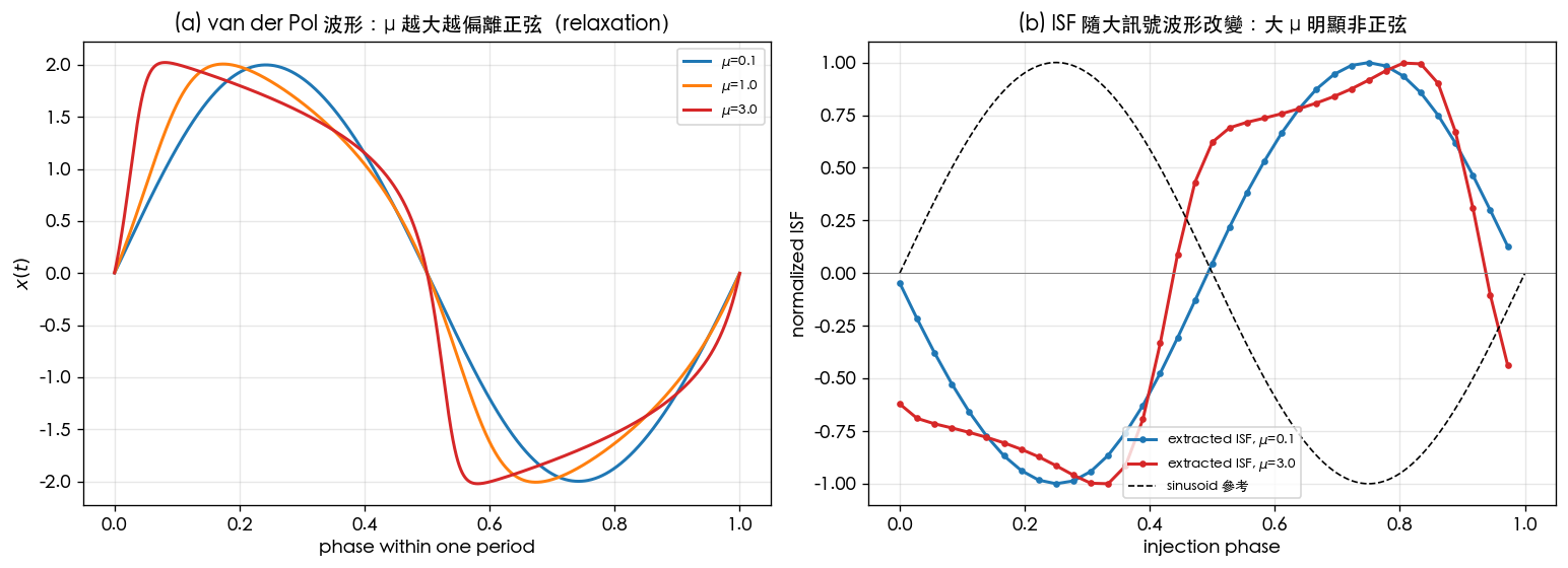
van der Pol waveforms (μ=0.1,1,3) and numerically extracted ISF (μ=0.1 near-sinusoidal, μ=3 clearly non-sinusoidal)

9. How to read the figure

Left panel (a), waveforms: $\mu=0.1$ (blue) is almost a sine; $\mu=1$ (orange) already shows visible asymmetry; $\mu=3$ (red) is classic relaxation — the rising segment is pushed fast and steep, the top flattens, the fall is abrupt too. The larger $\mu$ , the further the waveform departs from a sine.
Right panel (b), extracted ISF: at $\mu=0.1$ (blue) the measured ISF nearly overlaps the sine reference (black dashed), confirming "weak nonlinearity ≈ $\pm\sin$ "; at $\mu=3$ (red) the ISF is clearly deformed and asymmetric — the peak is shifted, rise/fall slopes are unequal, reflecting the steep edge in (a). The ISF changes with the large-signal waveform; it is not always $-\sin$ .
Key reading: panel (b) deliberately normalizes each ISF to peak 1, comparing shape only. The point is not the amplitude but that "the shape is no longer a clean sine". The more nonlinear the waveform, the richer the ISF harmonics ( $c_n$ beyond just $c_1$ ), and its $\Gamma_{rms}$ and $c_0$ (which sets $1/f^3$ ) are likewise dictated by the waveform.
Connection to rings: the ring's square-wave-like steep edges concentrate the ISF energy at the transitions, giving a shape close to a triangular pulse (lab_03) — another instance of "the large-signal waveform determines the ISF".

10. Corresponding paper equations/figures

Operational ISF definition (impulse → persistent phase step): [P1] Eq.(10), p.182, $h_\phi(t,\tau)=\Gamma(\omega_0\tau)/q_{max}\cdot u(t-\tau)$ .
"ISF is set by the waveform": [P1] Fig. 7, p.183 (LC vs ring waveforms with their ISFs); this lab uses van der Pol to display the waveform→ISF causality continuously.
Linearity of excess phase vs injected charge (small perturbation): [P1] Fig. 6, p.182.
ISF Fourier series (deformed ISF → more $c_n$ ): [P1] Eq.(12), p.183.
The van der Pol oscillator and the numerical ISF extraction method are external literature, not among the five source PDFs, supplemented from standard nonlinear-oscillation / oscillator perturbation literature (teaching toy). TODO: for a formal citation, add van der Pol (1927) and the adjoint/PSS ISF extraction methods.

11. Limitations and approximations

Toy model, not transistor-level: van der Pol is a dimensionless nonlinear oscillator for teaching; it does not correspond to any specific circuit; $x$ and time are normalized, with no physical V/A/s units.
Approximations of the numerical extraction: measuring the persistent time shift with a single small impulse assumes (i) $\Delta q$ is small enough for a linear response, (ii) the transient (amplitude perturbation) has decayed completely before $t_{late}$ , (iii) RK4 step size and zero-crossing interpolation errors are negligible. At large $\mu$ the time resolution at the steep edges gets strained, so the ISF is numerically more sensitive near the transitions.
Phase definition: the rising zero crossing serves as the phase reference; "phase" of a non-sinusoidal waveform is itself a matter of choice, and different reference points shift the ISF along its horizontal axis.
Phase only, no amplitude tracking: follows the [P1] first-order assumption (amplitude perturbations decay); AM–PM under strong nonlinearity is not fully captured.
Normalized amplitude: dividing the ISF by its peak in the figure is only for shape comparison; the absolute values of $\Gamma_{rms}$ and $c_0$ require keeping the $q_{max}$ normalization before plugging into [P1] Eq.(21)/(24).

Key takeaways

The ISF is set by the large-signal waveform, not always $-\sin$ : only near-sinusoidal oscillators approach $\pm\sin$ .
van der Pol: small $\mu$ → near-sinusoidal waveform, near-sinusoidal ISF; large $\mu$ → relaxation, deformed and asymmetric ISF.
Numerical extraction: inject a small impulse, measure the persistent steady-state time shift $\Delta t_{shift}$ , $\Delta\phi=-\omega_0\Delta t_{shift}$ , $\Gamma\approx\Delta\phi/\Delta q$ .
The more nonlinear the waveform → the more ISF harmonics → affecting $\Gamma_{rms}$ and $c_0$ (the latter sets $1/f^3$ upconversion).

1. Learning objectives​

2. Mathematical model​

3. Block diagram​

4. Core Python code​

5. Full script path​

6. Parameter table​

7. Unit table​

8. Simulation figure​

9. How to read the figure​

10. Corresponding paper equations/figures​

11. Limitations and approximations​

Key takeaways​

Further reading​