β: This English translation is in beta — the Traditional-Chinese original is the authoritative version.

Lab 14 — Cyclostationary noise and the effective ISF

Breadcrumb: Simulation labs › System & advanced › This page (cyclostationary / effective ISF). Upstream: lab_06, effective_isf; related: lab_09.

The previous labs all assumed the noise source is "equally noisy over the entire cycle" (stationary). Real circuits are not like that: a tail current source or a switching transistor conducts — and injects noise — only during part of the cycle. Noise whose intensity itself varies periodically with the oscillation phase is called cyclostationary noise. This lab uses a noise-modulating function (NMF) $\alpha(\theta)$, bounded between 0 and 1, to draw "when the device is noisy", then shows that what actually determines the phase noise is not the raw ISF but the effective ISF $\Gamma_{eff}=\Gamma\cdot\alpha$.

Physical intuition (conclusion first): phase noise depends not only on how noisy the device is ($\overline{i_n^2}$) but also on at which phase of the waveform it is noisy. For the same device, if its noisiest interval happens to land where the ISF is large (e.g. the zero crossing), it does a lot of damage; if it lands at the peak, where ISF≈0, little damage. Multiplying "when it is noisy", $\alpha(\theta)$, into the ISF gives $\Gamma_{eff}=\Gamma\alpha$; taking the rms of $\Gamma_{eff}$ then yields this cyclostationary source's true effective sensitivity $\Gamma_{eff,rms}$.

1. Learning objectives

• Understand the difference between stationary and cyclostationary noise.
• Model "the device is noisy only during part of the cycle" with the NMF $\alpha(\theta)\in[0,1]$.
• Derive the effective ISF $\Gamma_{eff}(\theta)=\Gamma(\theta)\,\alpha(\theta)$ and use it in place of $\Gamma$ when computing the rms.
• See that for the same device with the same amount of noise, the injection phase alone can change $\Gamma_{eff,rms}$ by severalfold.

2. Mathematical model

Start from the white-noise phase-noise law of [P1] Eq.(21), p.185:

$$\mathcal{L}\{\Delta\omega\}=10\log_{10}\!\left(\frac{\Gamma_{rms}^2}{q_{max}^2}\cdot\frac{\overline{i_n^2}/\Delta f}{4\,\Delta\omega^2}\right)$$

This assumes $\overline{i_n^2}/\Delta f$ is constant (stationary). If the noise is cyclostationary, its instantaneous PSD can be written as "a stationary component times a periodic gate":

$$\overline{i_n^2(\theta)}/\Delta f=\big(\overline{i_n^2}/\Delta f\big)\cdot\alpha^2(\theta),\qquad \alpha(\theta)\in[0,1].$$

Plugging this phase dependence back into the ISF integral kernel $\Gamma(\omega_0\tau)\,i_n(\tau)$ of [P1] Eq.(11), p.182 is equivalent to folding the noise's "$\alpha$" into the ISF. Define the effective ISF (spec section 10):

$$\Gamma_{eff}(\theta)=\Gamma(\theta)\,\alpha(\theta).$$

The phase noise of a cyclostationary source is then obtained by replacing $\Gamma_{rms}$ with $\Gamma_{eff,rms}$:

$$\Gamma_{eff,rms}=\sqrt{\frac{1}{2\pi}\int_0^{2\pi}\big[\Gamma(\theta)\,\alpha(\theta)\big]^2\,d\theta},$$

and substituting it into [P1] Eq.(21): $\mathcal{L}\propto\Gamma_{eff,rms}^2/q_{max}^2$.

• Why multiplication is correct: $\alpha$ describes "the fraction by which the noise amplitude is gated"; the ISF describes "how efficiently noise at that phase converts into phase". Both act on the same injection at the same instant, so their effects multiply.
• Dimension check: $\Gamma$ dimensionless, $\alpha$ dimensionless ($\in[0,1]$) ⇒ $\Gamma_{eff}$ dimensionless ✓, same units as the raw ISF, directly substitutable into Eq.(21).

This lab uses the ideal-LC $\Gamma(\theta)=-\sin\theta$ (derived in [P1]; maximum $\vert\Gamma\vert$ at the zero crossing $\theta=\pi/2$, $\Gamma\approx0$ at the peak $\theta=0$), paired with two smooth gates of equal width $\pi$: one gate at the zero crossing (bad), one at the peak (good).

3. Block diagram

4. Core Python code

Below is the core of simulations/lab_14_cyclostationary_isf.py: use gamma_lc_ideal ($-\sin$) as the ISF, a smooth periodic window nmf_window as $\alpha(\theta)$, then effective_isf (i.e. $\Gamma\cdot\alpha$) and gamma_rms to compute each rms.

import numpy as np
from simulations.common.isf_utils import gamma_lc_ideal, gamma_rms, effective_isf


def nmf_window(theta, center, width):
    """Smooth periodic gate in [0,1], centered at `center`, of given width (rad)."""
    d = np.angle(np.exp(1j * (theta - center)))  # wrapped distance
    return 0.5 * (1 + np.cos(np.pi * np.clip(d / (width / 2), -1, 1)))


theta = np.linspace(0, 2 * np.pi, 2000, endpoint=True)
gamma = gamma_lc_ideal(theta)                 # -sin(theta)

# case 1: device noisy near the ZERO CROSSING (where |Gamma| is max) -> bad
a_bad = nmf_window(theta, center=np.pi / 2, width=np.pi)
# case 2: device noisy near the PEAK (where |Gamma|~0) -> good
a_good = nmf_window(theta, center=0.0, width=np.pi)

g_bad = effective_isf(gamma, a_bad)           # Gamma * alpha
g_good = effective_isf(gamma, a_good)

grms = gamma_rms(theta, gamma)                # stationary reference
grms_bad = gamma_rms(theta, g_bad)
grms_good = gamma_rms(theta, g_good)
print(f"stationary={grms:.3f} bad={grms_bad:.3f} good={grms_good:.3f}")
# -> stationary=0.707, bad=0.395, good=0.177

effective_isf(gamma_values, alpha_values) is a pointwise product (see simulations/common/isf_utils.py), and gamma_rms(theta, gamma) is $\sqrt{\frac{1}{2\pi}\int_0^{2\pi}\Gamma^2\,d\theta}$, corresponding to [P1] Eq.(20).

5. Full script path

simulations/lab_14_cyclostationary_isf.py (main() generates the figure; the NMF uses nmf_window, the effective ISF and rms use effective_isf, gamma_rms, gamma_lc_ideal from simulations/common/isf_utils.py). Re-run: python scripts/run_all_sims.py.

6. Parameter table

Parameter	Symbol	Value	Role
ISF (ideal LC)	$\Gamma(\theta)$	$-\sin\theta$	fixed (physically derived)
Number of phase samples	—	2000	one cycle $[0,2\pi]$ (endpoint included)
Bad gate center	$\theta_{c,\text{bad}}$	$\pi/2$	noise lands on the zero crossing ($\vert\Gamma\vert$ maximal)
Good gate center	$\theta_{c,\text{good}}$	$0$	noise lands on the peak ($\Gamma\approx0$)
Gate width	width	$\pi$	same for both cases (half a cycle)
NMF bounds	$\alpha$	$[0,1]$	smooth raised-cosine window

7. Units table

Quantity	Symbol	Unit
Oscillation phase	$\theta=\omega_0\tau$	rad
ISF	$\Gamma$	dimensionless
NMF	$\alpha$	dimensionless ($\in[0,1]$)
effective ISF	$\Gamma_{eff}=\Gamma\alpha$	dimensionless
rms ISF	$\Gamma_{rms},\Gamma_{eff,rms}$	dimensionless

8. Simulation figure

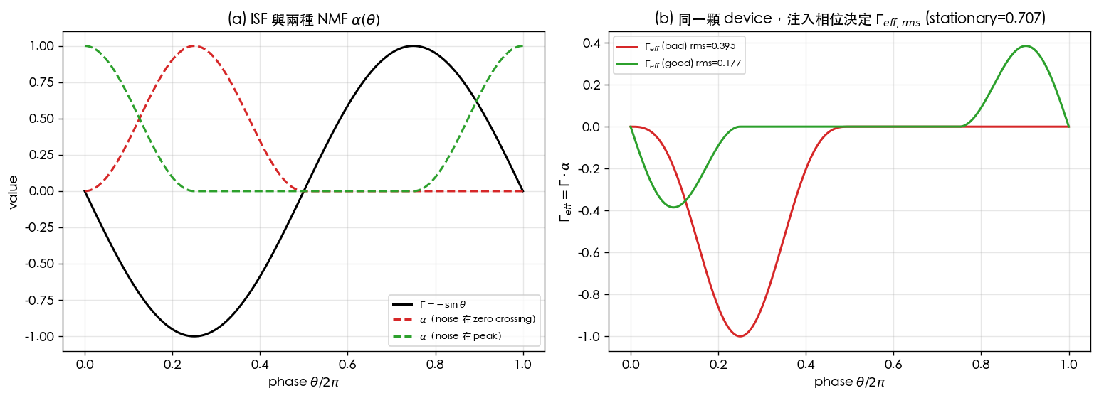
9. How to read the figure

• Left panel (a): the black curve is the ISF $\Gamma=-\sin\theta$ ($\vert\Gamma\vert$ maximal at $\theta/2\pi=0.25$, $0.75$, i.e. the zero crossings; $\Gamma=0$ at $0$, $0.5$, i.e. the peaks). The red dashed $\alpha$ places the device's noisy interval at the zero crossing ($\theta/2\pi\approx0.25$); the green dashed $\alpha$ places it at the peak ($\theta/2\pi\approx0$). The two gates have exactly the same shape and width — only the phase differs.
• Right panel (b): multiplying the left panel gives $\Gamma_{eff}=\Gamma\alpha$. The red curve (bad) collides with the ISF's large values at the zero crossing, leaving a deep, wide lobe, $\Gamma_{eff,rms}=0.395$; the green curve (good) lands on the peak, where the ISF is nearly 0, leaving only small residual lobes on either side, $\Gamma_{eff,rms}=0.177$.
• Key reading: the stationary reference is $\Gamma_{rms}=0.707$ (=$1/\sqrt2$, the full-cycle rms of $-\sin$). Once the gate is open for only half the cycle, the rms must drop; but how much it drops depends entirely on where the gate lands on the ISF: the bad case still retains $0.395$, the good case is cut to $0.177$ — a difference of about $2.2\times$. The phase-noise difference is $20\log_{10}(0.395/0.177)\approx7$ dB. Same device, same amount of noise — changing only the injection phase buys 7 dB.

10. Corresponding paper equations/figures

• White-noise phase noise (with $\Gamma_{eff,rms}$ replacing $\Gamma_{rms}$): [P1] Eq.(21), p.185.
• ISF integral kernel ($\Gamma\cdot i_n$, where $\alpha$ folds in): [P1] Eq.(11), p.182.
• Parseval / rms: [P1] Eq.(20), p.185, $\sum_n c_n^2=2\Gamma_{rms}^2$.
• Cyclostationary-noise concept: [P1] Sec. II-D "Cyclostationary Noise Sources", Eq.(25)–(27), p.186. There $i_n(t)=i_{n0}(t)\,\alpha(\omega_0 t)$ is Eq.(25), substituting it back into the integral is Eq.(26), and the effective ISF $\Gamma_{eff}(x)=\Gamma(x)\cdot\alpha(x)$ is Eq.(27); this lab is its toy visualization.
• Concept extension: where a device's $\alpha$ comes from and how it is mapped — see device_noise_mapping and effective_isf.

11. Limitations and approximations

• Toy model, not transistor-level: $\alpha(\theta)$ is an artificial raised-cosine window, not a real NMF extracted from a transistor's $g_m$ / conduction interval; the ISF is the ideal-LC $-\sin$. A real device's $\alpha$ and $\Gamma$ must both be extracted from PSS/transient simulation.
• $\Gamma_{eff}=\Gamma\alpha$ is a first-order approximation: assumes the noise amplitude is linearly modulated by the gate and that $\alpha$ and the phase response are mutually independent; ignores the noise's own AM–PM and any coupling between $\alpha$ and $\Gamma$.
• rms illustration only, no PSD run: this lab uses $\Gamma_{eff,rms}$ to show the scaling; it does not actually push a cyclostationary source through the [P1] Eq.(11) integral to produce a PSD (that would be an extension of lab_06).
• Single source: real circuits have multiple cyclostationary sources, each with its own $\alpha$; compute each $\Gamma_{eff,rms}$ separately and then sum in power.
• Factor-of-2: follows the $4\Delta\omega^2$ convention of Eq.(21); the factor-of-2 SSB bookkeeping difference does not affect any of the relative (dB) comparisons here.

Key takeaways

• Cyclostationary noise: noise intensity varies periodically with the oscillation phase, described by $\alpha(\theta)\in[0,1]$.
• Effective ISF: $\Gamma_{eff}=\Gamma\cdot\alpha$; the phase noise substitutes $\Gamma_{eff,rms}$ for $\Gamma_{rms}$ in [P1] Eq.(21).
• Numbers in this lab: stationary $\Gamma_{rms}=0.707$; noise at the zero crossing → $0.395$ (bad); at the peak → $0.177$ (good).
• Design implication: arranging noisy devices to inject at phases where the ISF is small (the peaks) saves considerable phase noise.

Further reading

• Effective-ISF theory: effective_isf
• White noise → phase noise (stationary version): lab_06_white_noise_phase_noise
• Design trade-off roundup: lab_09_design_tradeoffs
• Use in design/theory: how a device's $\alpha(\theta)$ is mapped from bias / conduction interval → device_noise_mapping