β: This English translation is in beta — the Traditional-Chinese original is the authoritative version.

Lab 36 — Lock-Acquisition Transient and Noise-Induced Cycle Slips

Prerequisites: injection_locking_noise (reduction of the [P3] generalized Adler equation to $\dot\theta=\Delta\omega-\omega_L\sin\theta$, in-lock noise shaping lab_26, out-of-lock pulling lab_27), paper_003 (origin of the lock characteristic), diffusion_dictionary (bookkeeping of the $D$ conventions) | Next: paper_004 (original source of the pull-in transient, [P4] Sec. V), quadrature_and_coupled_oscillators.

injection_locking_noise already answered the two steady-state questions — "after lock" (noise shaping) and "cannot lock" (pulling comb). This page fills in the two missing transient pieces:

What this page answers:

1. The moment the injection turns on, how long does the phase take to climb into the locked point? What is the settle rate? Why is it that near the lock-range edge you can "lock, but lock extremely slowly"? (Part a: the acquisition transient)
2. Once locked, what is the probability that noise occasionally kicks the phase over a whole cycle (a cycle slip — the phase slides by $2\pi$ in one event)? How does it scale with detuning and noise strength? At the canonical numbers, how often does it slip? (Part b)

Physical intuition (conclusion first): rewrite the Adler equation as an overdamped particle rolling in a tilted washboard potential and everything becomes obvious. Acquisition = the particle rolls down the slope into the nearest well: the potential curvature near the well is $\omega_c=\sqrt{\omega_L^2-\Delta\omega^2}$, so settling is an exponential with rate $\omega_c$; as the detuning ratio $r=\Delta\omega/\omega_L\to1$ the well and the saddle merge, the curvature vanishes, and the acquisition time diverges as $1/\sqrt{1-r}$ (critical slowing down). A cycle slip = thermal noise kicks the particle over the barrier of height $\Delta U$ next to the well and it slides down one washboard period ($2\pi$): the rate is Arrhenius-like, $e^{-\Delta U/D}$, and the "attempt frequency" is again the same $\omega_c/2\pi$ — the third appearance of that Pythagorean square root (first: settle rate; second: the noise-shaping corner of lab_26; outside lock it turns into the beat frequency $\omega_b$).

Positioning of this page: an advanced lab page with the theory derived in full on the page. The phase equation itself and the pull-in frequency are native results of [P3]/[P4] ([P3] Eq.(38)–(40), p.2115; [P4] Eq.(31)–(32) and Table I, p.2130, all verified against the original PDFs); the escape rate of noise over a barrier (Kramers/MFPT) is standard stochastic-process theory, not contained in the site's 5 PDFs (external references: Kramers 1940, Risken 1989, Ambegaokar–Halperin 1969, see the end of the page). This page honestly derives the barrier itself, quotes the escape-rate formula, and then checks everything against an SDE simulation term by term.

1. Teaching goals

• Solve $\dot\theta=\Delta\omega-\omega_L\sin\theta$ ($\lvert\Delta\omega\rvert\le\omega_L$) exactly by separation of variables + tan half-angle: the settle rate equals [P3] Eq.(40)'s pull-in frequency $\omega_c=\sqrt{\omega_L^2-\Delta\omega^2}$ not just in the linearization but globally.
• Demonstrate critical slowing down: sweep $r=\Delta\omega/\omega_L$ up to 0.99 and show the acquisition time diverging as $1/\omega_c$ (RK4 measurement vs the exact closed form, ratio 1.0000).
• Rewrite the Adler equation as the tilted-washboard potential $U(\theta)=-\Delta\omega\,\theta-\omega_L\cos\theta$ and derive step by step the forward barrier $\Delta U=2\omega_L[\sqrt{1-r^2}-r\arccos r]$ with its two limits ($r=0$: $2\omega_L$; $r\to1$: $\propto(1-r)^{3/2}$).
• Use the Kramers escape rate (external reference) to predict the slip rate $\nu\approx(\omega_c/2\pi)e^{-\Delta U/D}$, verified with a 512-walker Euler–Maruyama SDE: the log-linear slope = 0.993 of the analytic barrier, with the prefactor compared honestly (0.88).
• Map back to the canonical numbers ($f_L=5$ MHz, true-LC $S_n=0.5$ rad²/s): at $r=0.8$ the slip rate is $\sim10^{-1.86\times10^7}$ — it never happens; it only reaches once per second within $10^{-5}$ of the lock edge — thermal slips are a cliff, not a slope.

2. Mathematical model (theory derived on this page)

2.0 Starting point and notation (one-line recap)

The site-verified [P3] generalized Adler equation (Eq.(30), p.2113) reduces, for sinusoidal injection + the ideal-LC ISF, to the classic Adler equation (full derivation and symbol mapping in injection_locking_noise, Step 0):

$$\frac{d\theta}{dt}=\Delta\omega-\omega_L\sin\theta,\qquad \Delta\omega\equiv\omega_0-\omega_{inj}\ [\text{rad/s}],\quad \omega_L=\frac{I_{inj}}{2q_{max}}\ [\text{rad/s}].$$

([P3] itself writes it as $d\theta/dt=-\Delta\omega_{[P3]}+\Omega(\theta)$, Eq.(38), p.2115, with $\Delta\omega_{[P3]}=\omega_{inj}-\omega_0$ — an overall sign flip; this page's results depend only on $\Delta\omega^2$ and $r\equiv\Delta\omega/\omega_L$ and are unaffected.) Throughout we take $0\le r\le1$ ($\Delta\omega\ge0$) and often use dimensionless time $\tau=\omega_L t$ — the Adler dynamics depend only on $r$ and (in Part b) $D/\omega_L$; converting back to real units is a division by $\omega_L$.

2.1 Part (a): acquisition transient — exact solution and critical slowing

Step 1: locked point and linearization ([P3]'s native result). Steady state $\sin\theta_{ss}=r$, stable branch $\theta_{ss}=\arcsin r$ ($\cos\theta_{ss}\gt0$), unstable solution $\theta_u=\pi-\arcsin r$ (the stability criterion of [P3] Eq.(38)–(39), p.2115: $\Omega'(\theta_0)\lt0$). First-order Taylor expansion around $\theta_{ss}$ ($\sin\theta\approx r+\cos\theta_{ss}\,\delta\theta$):

$$\frac{d(\delta\theta)}{dt}=-\omega_c\,\delta\theta,\qquad \omega_c\equiv\omega_L\cos\theta_{ss}=\sqrt{\omega_L^2-\Delta\omega^2}.$$

This is exactly the pull-in frequency defined in [P3] Eq.(40), p.2115: $\omega_p:=-\Omega'(\theta_0)=1/\tau_p$, and [P3] states the solution is the exponential decay $\hat\theta(t)\propto e^{-t/\tau_p}$. Unit check: $[\omega_c]=$ rad/s ✓; $\delta\theta$ [rad] ÷ s = rad/s ✓.

Step 2: no linearization — solve exactly (separation of variables + tan half-angle). Separate time out:

$$t=\int\frac{d\theta}{\Delta\omega-\omega_L\sin\theta}.$$

Use the Weierstrass half-angle substitution $u=\tan(\theta/2)$ ($\sin\theta=\dfrac{2u}{1+u^2}$, $d\theta=\dfrac{2\,du}{1+u^2}$) — the exact same step used for the beat frequency in injection_locking_noise Part B — and the denominator becomes the same quadratic:

$$t=\int\frac{2\,du}{\Delta\omega\,u^2-2\omega_L u+\Delta\omega}.$$

The only difference is the sign of the discriminant: outside lock ($\Delta\omega\gt\omega_L$) it is negative, completing the square gives $\arctan$ → a periodic solution (beat frequency $\omega_b$); inside lock ($\Delta\omega\lt\omega_L$) the discriminant $4(\omega_L^2-\Delta\omega^2)\gt0$ and the quadratic has two real roots:

$$u_\pm=\frac{\omega_L\pm\omega_c}{\Delta\omega},\qquad u_+u_-=\frac{\omega_L^2-\omega_c^2}{\Delta\omega^2}=1 .$$

These two roots are none other than the half-angle tangents of the two equilibria — using the half-angle formula and $\Delta\omega^2=(\omega_L+\omega_c)(\omega_L-\omega_c)$ (rationalizing in the last step):

$$\tan\frac{\theta_{ss}}{2}=\frac{\sin\theta_{ss}}{1+\cos\theta_{ss}} =\frac{\Delta\omega}{\omega_L+\omega_c}=\frac{\omega_L-\omega_c}{\Delta\omega}=u_-\ (\text{stable}), \qquad u_+=\tan\frac{\theta_u}{2}\ (\text{unstable});$$

and $u_+u_-=1$ means $\tan\frac{\theta_{ss}}{2}\tan\frac{\theta_u}{2}=1\Leftrightarrow\theta_{ss}+\theta_u=\pi$ ✓ (self-consistent). Partial fractions ($u_+-u_-=2\omega_c/\Delta\omega$):

$$\frac{2}{\Delta\omega(u-u_+)(u-u_-)} =\frac{1}{\omega_c}\left[\frac{1}{u-u_+}-\frac{1}{u-u_-}\right] \quad\Longrightarrow\quad t=\frac{1}{\omega_c}\ln\left\lvert\frac{u-u_+}{u-u_-}\right\rvert+C.$$

Arrange into the cleanest form — define the trajectory coordinate $R$, which decays strictly exponentially:

$$\boxed{\ R(\theta)\equiv\frac{\tan\frac{\theta}{2}-\tan\frac{\theta_{ss}}{2}}{\tan\frac{\theta}{2}-\tan\frac{\theta_u}{2}}, \qquad R\big(\theta(t)\big)=R(\theta_0)\,e^{-\omega_c t}\ }$$

Unit check: $u$, $R$ dimensionless; the exponent $\omega_c t=$ (rad/s)(s) = rad (dimensionless) ✓. Three readouts:

1. The settle rate is $\omega_c$ globally — not only in the linearization: the whole trajectory converges as $e^{-\omega_c t}$ in the $R$ coordinate; near the locked point $u-u_-\propto e^{-\omega_c t}$, recovering Step 1 ✓.
2. Exact acquisition time (from $\theta_0$ to $\theta_{ss}-\varepsilon$): $T_{acq}=\dfrac{1}{\omega_c}\ln\dfrac{R(\theta_0)}{R(\theta_{ss}-\varepsilon)}$ — $1/\omega_c$ is the protagonist; the start point and the threshold enter only through the logarithm.
3. Equivalent to [P4] Eq.(31), p.2130. [P4] writes the same solution as $\tan(N\tilde\theta/2)=\tan(N\tilde\theta_0/2)\tanh\!\big((\omega_p t+\phi_0)/2\big)$ (its coordinate shifts the lock characteristic into an even function, so the unstable point sits exactly at $-\tilde\theta_0$). Using the identity $x=x_0\tanh z\Leftrightarrow\dfrac{x-x_0}{x+x_0}=-e^{-2z}$ this becomes the boxed $R$ form; the $/2$ inside the tanh argument cancels against the 2 of $e^{-2z}$, so the decay rate is still $\omega_p$ (= our $\omega_c$; [P4] Eq.(32): $\omega_p=N\sqrt{\omega_L^2-\Delta\omega^2}$ with $N=1$) — that 2 is tanh half-angle bookkeeping, not physics. Honest note: $\tanh$ only sweeps $(-1,1)$, so [P4]'s form covers initial conditions on the arc between the two equilibria; starting outside that arc the same solution family takes the $\coth$ branch with the identical rate — the $R$ form (any real $R(\theta_0)$) contains both branches. [P4] Table I, p.2130 validates this exponential pull-in with circuit simulations: $\tau_p/T_{inj}$ simulated 6 / 1.87 / 16.9 vs theory 5.95 / 1.79 / 17.4.

Step 3: critical slowing down (the price of the lock-range edge). Let $r=1-\delta$, $\delta\ll1$:

$$\omega_c=\omega_L\sqrt{1-r^2}=\omega_L\sqrt{\delta(2-\delta)}\approx\sqrt{2}\,\omega_L\sqrt{1-r}\ \to\ 0,$$ $$T_{acq}\approx\frac{1}{\omega_c}\Big[\ln\frac{1}{\varepsilon}+O(1)\Big]\ \propto\ \frac{1}{\sqrt{1-r}}\ \to\ \infty .$$

Physics: as $r\to1$ the stable point $\arcsin r$ and the unstable point $\pi-\arcsin r$ merge at $\pi/2$ (a saddle-node bifurcation) and the restoring slope vanishes — "can lock" and "locks fast" are two different things. (Saddle-node critical slowing is a standard nonlinear-dynamics result — external reference, not among the site's 5 PDFs, e.g. S. H. Strogatz, Nonlinear Dynamics and Chaos, 2nd ed., Westview, 2015 — but the derivation above is self-contained.) This echoes the two steady-state conclusions of injection_locking_noise: at the edge the noise-suppression corner $\omega_c\to0$ (Part A) and, outside lock, the beat frequency $\omega_b\to0$ (Part B) — one square root, three kinds of slowing.

Example (acquisition time, canonical scale): $f_L=\omega_L/2\pi=5$ MHz, $r=0.5$, $\theta_0=0$, $\varepsilon=0.01$ rad. The simulation (Section 8) measures $\omega_L T_{acq}=4.435$, so in real units $T_{acq}=4.435/(2\pi\times5\times10^6)=141.2$ ns — 706 periods of the $f_0=5$ GHz carrier. Dimension check: dimensionless ÷ (rad/s) = s ✓. Same procedure at $r=0.99$: $\omega_L T_{acq}=22.913\Rightarrow729.3$ ns (3647 periods) — pushing the detuning from half to the edge slows acquisition by a factor of 5.2, and it keeps degrading as $1/\sqrt{1-r}$.

2.2 Part (b): tilted washboard, barrier, and Kramers escape

Step 1: put the noise back and rewrite as a gradient flow. The oscillator's own white noise, averaged through the ISF, is an effective white-FM drive $n(t)$ (one-sided PSD $S_n=\Gamma_{rms}^2\,\overline{i_n^2}/\Delta f\,/q_{max}^2$ [rad²/s], derived in injection_locking_noise, Step 2):

$$\frac{d\theta}{dt}=\Delta\omega-\omega_L\sin\theta+n(t) =-\frac{\partial U}{\partial\theta}+n(t),\qquad \boxed{\ U(\theta)=-\Delta\omega\,\theta-\omega_L\cos\theta\ }$$

(Check: $-\partial_\theta U=\Delta\omega-\omega_L\sin\theta$ ✓.) This is the tilted washboard: mean slope $-\Delta\omega$ (the detuning tilts the whole potential downhill) plus a ripple of amplitude $\omega_L$ (the injection's restoring force). Units: $[\Delta\omega\,\theta]=$ (rad/s)(rad), $[\omega_L\cos\theta]=$ rad/s — rad is dimensionless (site convention), so both terms are $\text{rad}^2/\text{s}$, equivalently $1/\text{s}$ ✓; $U'$ is rad/s, same units as $\dot\theta$ ✓.

Convention flag (the 2 and the 4 in $D$, following diffusion_dictionary): the Kramers literature writes the noise as $\langle n(t)n(t')\rangle=2D\,\delta(t-t')$ — this is convention B ($\mathrm{Var}[\Delta\phi]=2D\lvert t\rvert$). The autocorrelation of a one-sided PSD $S_n$ is $(S_n/2)\delta$ (this 2 = one-sided↔two-sided Wiener–Khinchin), and matching to $2D\delta$ absorbs the second 2 (convention-B definition), so

$$D=\frac{S_n}{4}=\frac{\kappa^2}{2}=\frac{\Gamma_{rms}^2}{4q_{max}^2}\frac{\overline{i_n^2}}{\Delta f}\quad[\text{rad}^2/\text{s}].$$

Canonical: true LC ($\Gamma_{rms}=1/\sqrt2$, $S_i=10^{-24}$ A²/Hz, $q_{max}=1$ pC) $S_n=0.5\Rightarrow D=0.125$ rad²/s; representative $\Gamma_{rms}=0.5$ gives $S_n=0.25\Rightarrow D=0.0625$ rad²/s. (The same representative numbers on a free-running oscillator correspond to $\mathcal{L}(1\text{MHz})=-148.0$ dBc/Hz — the SSB $/4$ convention of [P1] Eq.(21); the time-domain $/2$ convention gives $-145.0$ dBc/Hz. The identity of every 2/4 is audited in diffusion_dictionary.)

Step 2: the barrier $\Delta U$ — computed honestly. Extrema: $U'(\theta)=0\Leftrightarrow\sin\theta=r$. Well bottom $\theta_{ss}=\arcsin r$ ($U''=\omega_L\cos\theta_{ss}=+\omega_c\gt0$), barrier top $\theta_u=\pi-\arcsin r$ ($U''=-\omega_c$) — the same pair of equilibria, the same $\omega_c$ again. The height to climb sliding forward (down the tilt, $\theta$ increasing):

$$\begin{aligned} \Delta U_+&=U(\theta_u)-U(\theta_{ss})\\ &=\big[-\Delta\omega(\pi-\arcsin r)+\omega_L\sqrt{1-r^2}\big] -\big[-\Delta\omega\arcsin r-\omega_L\sqrt{1-r^2}\big]\\ &=2\omega_L\sqrt{1-r^2}-\Delta\omega\big(\pi-2\arcsin r\big)\\ &=2\omega_L\Big[\sqrt{1-r^2}-r\Big(\tfrac{\pi}{2}-\arcsin r\Big)\Big] \end{aligned}$$

Using $\tfrac{\pi}{2}-\arcsin r=\arccos r$:

$$\boxed{\ \Delta U_+(r)=2\,\omega_L\Big[\sqrt{1-r^2}-r\arccos r\Big]\ }$$

(The 2 here is geometric — max minus min each contribute one $\omega_L\sqrt{1-r^2}$ — not a bookkeeping convention.) Three checks:

• Units: $\omega_L$ [rad/s] × dimensionless = rad²/s (rad≡1 bookkeeping as above); the exponent $\Delta U/D=$ (rad²/s)/(rad²/s) is dimensionless ✓.
• $r=0$: $\Delta U_+=2\omega_L$ — valley-to-peak of the untilted washboard $-\omega_L\cos\theta$ ✓; then forward/backward are symmetric, slips are equally likely in both directions, and the net drift is zero.
• $r\to1$ ($r=1-\delta$): $\sqrt{1-r^2}\approx\sqrt{2\delta}(1-\delta/4)$, $\arccos r\approx\sqrt{2\delta}(1+\delta/12)$, and the leading term of the difference is $\Delta U_+\approx\dfrac{4\sqrt2}{3}\,\omega_L(1-r)^{3/2}\to0$ — the standard saddle-node barrier scaling. Plugging $r=0.8$ into the asymptote gives $0.169\,\omega_L$, only 1% off the exact $0.1704\,\omega_L$.

Backward barrier: sliding backwards means climbing the barrier at $\theta_u-2\pi$, one extra full period of tilt: $\Delta U_-=\Delta U_++2\pi\Delta\omega$ (the net potential drop per period is $U(\theta-2\pi)-U(\theta)=2\pi\Delta\omega$). At $r=0.8$ the backward rate is suppressed by an extra $e^{-2\pi r\,\omega_L/D}$ — utterly negligible at this page's parameters, so slips are effectively one-directional (toward the detuning).

Step 3: the escape rate (Kramers — external reference, honestly flagged). For the overdamped SDE $\dot x=-U'(x)+n$, $\langle nn'\rangle=2D\delta$, and barrier $\Delta U\gg D$, the mean escape rate is

$$\nu=\frac{\sqrt{U''(\theta_{ss})\,\lvert U''(\theta_u)\rvert}}{2\pi}\,e^{-\Delta U/D} \qquad\text{(Kramers 1940; Risken 1989, Ch. 11 — external references, not among the site's 5 PDFs)}$$

In this problem $U''(\theta_{ss})=\lvert U''(\theta_u)\rvert=\omega_c$, so

$$\boxed{\ \nu_{slip}\approx\frac{\omega_c}{2\pi}\,e^{-\Delta U_+/D}\ } \qquad\Big[\frac{1}{\text{s}}\Big]$$

Dimension check: $\omega_c/2\pi$ = rad/s ÷ rad = 1/s (attempt frequency, Hz) ✓, the exponent dimensionless ✓. The third appearance of $\omega_c$: in-lock settle rate, noise-shaping corner (lab_26), and now the escape attempt rate — all of them are the slope of the lock characteristic at the locked point. The same tilted-washboard-plus-thermal-escape mathematics also governs the RSJ model of Josephson junctions and the overdamped pendulum (Ambegaokar–Halperin 1969, external reference) — the Adler equation is simply its oscillator incarnation. Honest boundary: the Kramers formula is the asymptote for $\Delta U/D\gg1$; at moderate barriers there are $O(D/\Delta U)$ corrections — hence Section 8 uses the slope (the barrier) as the primary verification and reports the prefactor deviation honestly.

Example (slip rate, canonical numbers): $f_L=5$ MHz, $r=0.8$. $\Delta U_+=0.1704\,\omega_L=0.1704\times2\pi\times5\times10^6=5.353\times10^6$ rad²/s; $\omega_c=0.6\,\omega_L$ (a 3–4–5 triangle), attempt frequency $\omega_c/2\pi=3.0$ MHz. True-LC thermal noise $D=0.125$ rad²/s: $\Delta U/D=4.283\times10^7$, $\log_{10}\nu\approx6.5-4.283\times10^7\times0.4343=-1.86\times10^7$ — a slip rate of $10^{-18{,}600{,}000}$ per second. The age of the universe is only $4\times10^{17}$ s: it never happens. Asking the question backwards — "how close to the edge before it slips once per second" — solving $\nu(r^\*)=1$ gives $1-r^\*=7.6\times10^{-6}$ (true LC; the representative $D=0.0625$ gives $4.7\times10^{-6}$) — the detuning must sit within seven parts per million of the lock-range edge. Conclusion: for clean injection + thermal noise, cycle slips are not a gradual degradation but a cliff; the slips seen in practice almost always come from transients, interferers, or loops whose effective $D$ is far larger (low-SNR CDRs, bang-bang PLLs) — and at the cliff edge $\omega_c$ has already collapsed (at $r^\*$ the noise-shaping corner is down to 19.5 kHz — it gets dirty before it slips). The cost of one slip: the phase advances by $\pm2\pi$ in one go = one whole carrier period — a forwarded-clock SerDes drops a bit outright, a counting PLL miscounts a beat, so it is a "rate" to be suppressed exponentially, not an "amplitude" that averages out.

2.3 Applicability and failure conditions

Condition	When it holds	What happens when it fails
Weak injection $I_{inj}\ll I_{max}=\omega_0q_{max}$ ([P3] Eq.(36)–(37), p.2115)	Adler / lock characteristic linear in $i_{inj}$	Strong injection: needs [P4]'s APF/AM corrections (paper_004)
$\theta$ slowly varying (≈ constant within one period)	Time-averaged equation ([P3] Eq.(30)) valid	If $\dot\theta\sim\omega_{inj}$ early in acquisition, the averaging fails (here $\omega_c\ll\omega_{inj}$, no problem)
Sinusoidal injection + ideal-LC ISF	The $-\omega_L\sin\theta$ closed form, real roots $u_\pm$	Arbitrary waveform/topology: back to $\Omega(\theta)$; settle rate generalizes to $-\Omega'(\theta_{ss})$ ([P3] Eq.(40)), the barrier becomes the corresponding area of $\int[\Omega(\theta)-\Delta\omega]d\theta$, no simple closed form
Pure phase model (amplitude dynamics ignored)	Everything on this page	Large transients / strong injection in LC: amplitude moves too, [P4] Sec. V APF corrections (the third column of Table I is exactly an APF case)
$\Delta U\gg D$ (high barrier)	Kramers rate with prefactor $\omega_c/2\pi$	Moderate/low barrier: the exponential slope still approximates, the prefactor deviates more (Section 8 measures 0.77–0.94); for $\Delta U\lesssim D$ it fails entirely — continuous sliding, i.e. pulling
White-FM drive	$D=S_n/4$ constant	Flicker FM: $D$ is no longer constant, escape statistics non-Poisson (not covered here)

3. Block diagram

4. Python core code

Excerpted from simulations/lab_36_lock_acquisition.py (checked against the source). Exact closed form, barrier, and the slip-counting main loop:

def barrier(r):                        # ΔU/ω_L = 2(√(1−r²) − r·arccos r)
    return 2.0 * (np.sqrt(1.0 - r**2) - r * np.arccos(r))

def acquisition_exact(r, theta0=0.0, eps=0.01):
    wc = np.sqrt(1.0 - r**2)           # ω_c/ω_L (dimensionless pull-in rate)
    um = (1.0 - wc) / r                # tan(θ_ss/2) (stable root)
    up = (1.0 + wc) / r                # tan(θ_u/2)  (unstable root; um·up = 1)
    R = lambda u: (u - um) / (u - up)  # R(θ(t)) = R(θ₀)·e^(−ω_c t)
    u0, uthr = np.tan(theta0 / 2), np.tan((np.arcsin(r) - eps) / 2)
    return (1.0 / wc) * np.log(R(u0) / R(uthr))   # exact acquisition time [1/ω_L]

# --- slips: Euler–Maruyama (dimensionless τ=ω_L t; n supplied by the site's white_noise) ---
# white_noise one-sided PSD = 4D ⇒ increment variance 2·D·dτ (convention B ⟨nn'⟩=2Dδ) [checked]
nz = white_noise(nb * m, 4.0 * D, 1.0 / dtau, rng).reshape(nb, m)
for i in range(nb):
    theta += (r - np.sin(theta) + nz[i]) * dtau
# integer slip count: floor((θ−θ_u)/2π) is constant inside one well, jumps ±1 on a slip
slips = int(np.sum(np.floor((th_end - th_u) / (2*np.pi))
                   - np.floor((th_start - th_u) / (2*np.pi))))

Verification numbers as printed (PYTHONPATH=. python3 simulations/lab_36_lock_acquisition.py):

print(ratio_min, ratio_max)     # -> 1.0000 1.0000 RK4 acquisition time / exact closed form (all 12 r values)
print(T_r050)                   # -> 4.435 ω_L·T_acq @ r=0.5 (ε=0.01 rad, θ₀=0)
print(T_r090)                   # -> 9.202 ω_L·T_acq @ r=0.9
print(T_r099)                   # -> 22.913 ω_L·T_acq @ r=0.99 (critical slowing)
print(wc_T_range)               # -> 2.30 .. 4.10 ω_c·T_acq barely moves (the divergence is all in 1/ω_c)
print(max_traj_dev)             # -> 2.90e-14 rad, max deviation closed form vs RK4 whole trajectory (r=0.8)
print(T_r05_real)               # -> 141.2 ns (=706 carrier periods at 5 GHz; f_L=5 MHz)
print(dU_over_wL)               # -> 0.1704 barrier ΔU/ω_L @ r=0.8
print(slips_x6, ratio_x6)       # -> 1350, 0.93 slips and (measured/Kramers) @ ΔU/D=6
print(dU_fit_over_theory)       # -> 0.993 fitted barrier / analytic barrier (log-linear slope)
print(prefac_fit_over_kramers)  # -> 0.88 fitted prefactor / (ω_c/2π) (Kramers asymptote)
print(dt_halving)               # -> 1.053 slip-rate ratio after halving dτ (step-size bias ~5%)
print(log10_nu_canonical)       # -> -1.860e7 log10(ν·s) @ true-LC D=0.125, r=0.8
print(one_minus_rstar)          # -> 7.573e-06 1−r*: distance to the edge for ν=1 slip/s (true LC)

5. Full script path

simulations/lab_36_lock_acquisition.py (depends on white_noise from simulations/common/noise_utils.py, savefig from simulations/common/plot_utils.py; scipy.optimize.brentq solves for $r^\*$).

Run: PYTHONPATH=. python3 simulations/lab_36_lock_acquisition.py (about 27 s on one machine; fixed seed default_rng(36), fully reproducible).

6. Parameter table

Parameter	Variable	Value	Meaning
Half lock range	F_LOCK	5.0 MHz	$f_L=\omega_L/2\pi$ (for real-unit conversion)
Carrier	F0	5 GHz	canonical $f_0$ (only for period-count conversion)
Detuning sweep	r_arr	0.10–0.99 (12 points)	Part (a): $r=\Delta\omega/\omega_L$
Settle threshold	EPS	0.01 rad	acquisition declared at $\theta_{ss}-\varepsilon$
RK4 step	dtau	0.002	dimensionless $\tau=\omega_L t$; threshold via linear interpolation
Slip detuning	R_SLIP	0.8	Part (b) fixed ($\omega_c=0.6\,\omega_L$, 3–4–5)
Barrier/noise ratio	x_list	4–9 (6 points)	$\Delta U/D$; $D=\Delta U/x$ solved backwards
Walkers	M	512	parallel SDE samples
EM steps/step size	NSTEPS/DTAU	$6\times10^5$ / 0.02	per walker $\tau_{tot}=12000$; total $\tau=6.1\times10^6$
Noise	white_noise(…,4D,1/dτ)	—	convention B $\langle nn'\rangle=2D\delta$ (increment variance $2D\,d\tau$)
Canonical $D$	D_TRUE_LC/D_REPR	0.125 / 0.0625 rad²/s	$S_n/4$ (true LC / representative)

7. Unit table

Quantity	Symbol	Units	Notes
Phase difference	$\theta$	rad	oscillator phase relative to the injection
Detuning / half lock range	$\Delta\omega$, $\omega_L$	rad/s	$r=\Delta\omega/\omega_L$ dimensionless
Pull-in rate	$\omega_c=\sqrt{\omega_L^2-\Delta\omega^2}$	rad/s	the $\omega_p$ of [P3] Eq.(40)
Acquisition time	$T_{acq}$	s	figure uses dimensionless $\omega_L T_{acq}$
Washboard potential	$U(\theta)$	rad²/s	rad dimensionless, equivalent to $1/\text{s}$
Barrier	$\Delta U_+$	rad²/s	$=2\omega_L[\sqrt{1-r^2}-r\arccos r]$
White-FM drive	$n(t)$, $S_n$	rad/s, rad²/s	one-sided PSD
Diffusion constant (convention B)	$D=S_n/4$	rad²/s	$\langle nn'\rangle=2D\delta$
Slip rate	$\nu$	1/s	dimensionless version $\nu/\omega_L$ (per unit $\omega_L t$)

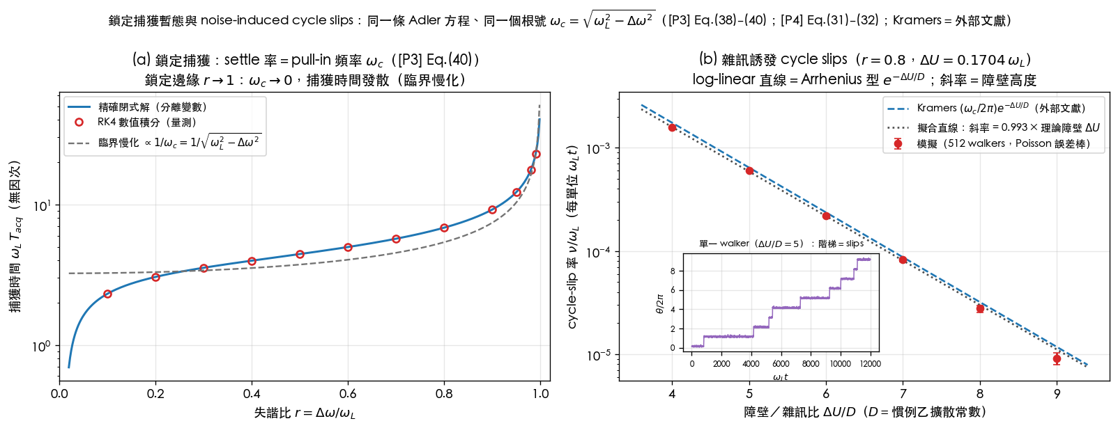
8. Simulation figure

9. How to read the figure

(a) Acquisition time (left): the blue line is the exact closed form $T_{acq}=\omega_c^{-1}\ln[R(\theta_0)/R(\theta_{ss}-\varepsilon)]$, the red circles are the first-crossing times measured by direct RK4 integration — all 12 values of $r$ agree to a ratio of 1.0000 (maximum deviation over the whole trajectory $2.9\times10^{-14}$ rad, machine-precision level: the closed form is the solution). The gray dashed line is the pure $1/\omega_c$ scaling (anchored at $r=0.99$): beyond $r\gtrsim0.5$ the measured points ride it exactly — every bit of the divergence comes from $\omega_c\to0$, while the start point and threshold enter only through the log ($\omega_c T_{acq}$ stays within 2.30–4.10 throughout, while $T_{acq}$ itself spans an order of magnitude). The design reading: the acquisition bandwidth and the noise-suppression bandwidth are the same number — pulling the detuning back from the edge ($r=0.99$) to mid-range ($r=0.5$) not only drops the noise plateau (the $1/\cos^2\theta_{ss}$ accounting of lab_26) but also makes acquisition 5.2× faster.

(b) Slip rate (right): on the log-linear axis the measured points fall on a straight line — the signature of an Arrhenius-type $e^{-\Delta U/D}$. The weighted fit of the slope gives $\Delta U_{fit}=0.993\,\Delta U_{theory}$: the barrier height is measured by the simulation itself, matching $2\omega_L[\sqrt{1-r^2}-r\arccos r]=0.1704\,\omega_L$. The prefactor, honestly: the fit gives 0.88 of the Kramers $\omega_c/2\pi$, with point-by-point ratios 0.77–0.94 — three sources: Kramers is the $\Delta U/D\gg1$ asymptote ($x=4$ is only a moderate barrier), Euler step-size bias (halving $d\tau$ moves the slip rate by 5.3%, dt_halving = 1.053), and statistics at $x=9$ with only 56 events (error bar ±13%). The exponent (the physics) is accurate to 0.7%; the prefactor (asymptotics + numerics) is off by a tenth — exactly what Kramers theory should look like. The inset shows a single walker's $\theta/2\pi$ at $\Delta U/D=5$: long plateaus (dithering inside a well) plus integer stair steps (one $2\pi$ slide per slip) — a slip is a discrete event, not a continuous drift; the plateau lengths are exponentially distributed, which is also why counting integer jumps of $\mathrm{floor}((\theta-\theta_u)/2\pi)$ is the cleanest method (constant inside a well, ±1 across the barrier, zero fractional noise).

10. Corresponding paper equations / figures

• Stability and pull-in (linearized settling): [P3] Eq.(38), p.2115 ($d\theta/dt=-\Delta\omega+\Omega(\theta)$), Eq.(39) ($d\hat\theta/dt=\Omega'(\theta_0)\hat\theta$), Eq.(40) ($1/\tau_p\equiv\omega_p:=-\Omega'(\theta_0)$, exponential decay $\hat\theta\propto e^{-t/\tau_p}$); Fig. 8, p.2115 (decomposition of the ISF harmonics into $\omega_p$), Fig. 9, p.2115 (feedback block diagram). This page's $\omega_c$ = that $\omega_p$ specialized to sinusoidal + ideal-LC: $\sqrt{\omega_L^2-\Delta\omega^2}$.
• Exact pull-in closed form: [P4] Sec. V-A "Pull-In Process", Eq.(31), p.2130 (tanh form; the $R$ form of Section 2.1 Step 2 is equivalent and also covers the coth branch), Eq.(32), p.2130 ($\omega_p=N\sqrt{\omega_L^2-\Delta\omega^2}$ — the Pythagorean twin of the out-of-lock $\omega_b$ of Eq.(34)); Table I, p.2130 (circuit-simulated $\tau_p/T_{inj}$ vs theory: 6/5.95, 1.87/1.79, 16.9/17.4 — the original validation of exponential pull-in).
• Weak-injection linearity boundary: [P3] Eq.(36)–(37), p.2115 ($I_{inj}\ll I_{max}:=\omega_0q_{max}$).
• Where the noise step belongs: [P4] p.2130 states that the noise analysis of free-running and injection-locked oscillators via the pulling equation is deferred to its reference [29, Ch. 7] (Hong's PhD thesis) — attaching $n(t)$ to Adler and reading off the slip rate via Kramers is not in the site's 5 PDFs; this page derives the barrier itself, quotes the standard escape rate (external references), and checks it against simulation.
• Upstream machinery: $S_n=\Gamma_{rms}^2 S_i/q_{max}^2$ comes from the time-domain derivation of [P1] Eq.(11)/(21) (white_noise_to_phase_noise); the $D=S_n/4$ bookkeeping is audited in diffusion_dictionary (the $\kappa^2=2D$ of [P2] Eq.(11)/(12)).

11. Limitations and approximations

• Phase-domain toy model: what is integrated is the time-averaged Adler equation (the sinusoidal reduction of [P3] Eq.(30)), not a transistor-level circuit — no amplitude dynamics (APF), no harmonics, no cyclostationary weighting (the latter is already absorbed into $S_n$ through $\Gamma_{rms}$, see effective_isf).
• Kramers asymptotics: $\nu=(\omega_c/2\pi)e^{-\Delta U/D}$ holds only for $\Delta U\gg D$; this lab sweeps $\Delta U/D=4$–$9$, medium-to-high barriers, so the exponential slope is accurate (0.993) while the prefactor is off by 12%. Higher accuracy needs the closed-form MFPT double integral (Risken Ch. 11), not expanded here.
• Euler–Maruyama, first-order weak convergence: at $d\tau=0.02$ the slip-rate step-size bias is ~5% (measured dt_halving = 1.053); the barrier fit is insensitive to it (the slope is a difference between ratios).
• One-directional counting assumption: at $r=0.8$ the backward barrier is higher by $2\pi r\,\omega_L$, suppressing the backward rate by $e^{-2\pi r\omega_L/D}$ ($\lesssim e^{-100}$ at this page's parameters); at small $r$ or large $D$ forward and backward slips must be counted separately.
• White-noise assumption: under flicker FM, $D$ is not constant and slips are non-Poissonian; long-gate slip statistics in measurements then deviate from exponential.
• $T_{acq}$ depends on the start point: $\theta_0=0$ is a representative choice; changing it only moves the log factor (the 2.30–4.10 range of $\omega_c T$), never the $1/\omega_c$ divergence. Starting exactly at $\theta_u$ (measure zero) never acquires, in theory.

Key takeaways

• The in-lock Adler equation has an exact closed-form solution: $R(\theta)\equiv\dfrac{\tan\frac{\theta}{2}-\tan\frac{\theta_{ss}}{2}}{\tan\frac{\theta}{2}-\tan\frac{\theta_u}{2}}$ decays strictly as $e^{-\omega_c t}$, so the settle rate is globally the pull-in frequency $\omega_c=\sqrt{\omega_L^2-\Delta\omega^2}$ ([P3] Eq.(40); equivalent to the tanh form of [P4] Eq.(31)–(32)).
• Critical slowing: as $r\to1$ the two equilibria merge in a saddle-node, $T_{acq}\propto(1-r)^{-1/2}$; simulation: $\omega_L T_{acq}$ grows from 4.435 ($r=0.5$) to 22.913 ($r=0.99$), all riding the $1/\omega_c$ line (RK4/closed-form ratio 1.0000). Canonical scale: 141.2 ns → 729.3 ns.
• With white FM noise the Adler equation = an overdamped particle in the tilted washboard $U=-\Delta\omega\theta-\omega_L\cos\theta$; forward barrier $\Delta U_+=2\omega_L[\sqrt{1-r^2}-r\arccos r]$ ($r{=}0.8$: $0.1704\,\omega_L$; $r\to1$: $\propto(1-r)^{3/2}$).
• Kramers slip rate $\nu\approx(\omega_c/2\pi)e^{-\Delta U_+/D}$ (external reference), $D=S_n/4$ (convention B): the simulated log-linear slope = 0.993 of the barrier, prefactor 0.88 (asymptotics + Euler, honestly accounted).
• Canonical numbers ($f_L=5$ MHz, true-LC $D=0.125$ rad²/s, $r=0.8$): $\log_{10}\nu\approx-1.86\times10^7$ — thermal slips never happen; one slip per second requires pushing the detuning to the cliff edge $1-r=7.6\times10^{-6}$. One slip = one whole carrier period — a dropped-bit-class event.
• The four identities of the same square root $\sqrt{\lvert\omega_L^2-\Delta\omega^2\rvert}$: in lock, settle rate = noise-shaping corner = Kramers attempt frequency; out of lock, the beat frequency $\omega_b$.

Further reading

• injection_locking_noise: the steady-state prequel — in-lock noise shaping (lab_26), out-of-lock pulling comb (lab_27), the same $\omega_c$.
• paper_003: generalized Adler, lock characteristic, stability ([P3] Eq.(26)–(40)).
• paper_004: original source of the pull-in transient and the beat frequency ([P4] Sec. V, Eq.(31)–(34), Table I).
• diffusion_dictionary: $\kappa^2$, the two $D$ conventions, linewidth — the audit behind this page's $D=S_n/4$.
• lorentzian_linewidth: phase diffusion of the free-running oscillator — without a washboard, $D$ turns directly into linewidth.
• lab_13: acquisition/tracking of second-order loops — the PLL version of the same set of questions.

External references (not among the 5 downloaded PDFs)

• [E-Kramers] H. A. Kramers, "Brownian motion in a field of force and the diffusion model of chemical reactions," Physica, vol. 7, no. 4, pp. 284–304, 1940. (Original source of the overdamped escape rate $\propto e^{-\Delta U/D}$ with the curvature prefactor.)
• [E-Risken] H. Risken, The Fokker–Planck Equation: Methods of Solution and Applications, 2nd ed., Springer, 1989, Ch. 11. (Complete MFPT theory of tilted periodic potentials.)
• [E-AH] V. Ambegaokar and B. I. Halperin, "Voltage due to thermal noise in the dc Josephson effect," Phys. Rev. Lett., vol. 22, no. 25, pp. 1364–1366, 1969. (The classic application of the same tilted-washboard + thermal-escape mathematics to Josephson junctions.)
• [E-Strogatz] S. H. Strogatz, Nonlinear Dynamics and Chaos, 2nd ed., Westview, 2015. (The standard textbook for saddle-node bifurcations and critical slowing $\propto1/\sqrt{\text{distance}}$.)
• [E-Adler] R. Adler, "A Study of Locking Phenomena in Oscillators," Proc. IRE, vol. 34, no. 6, pp. 351–357, Jun. 1946. (The classic Adler equation.)