β: This English translation is in beta — the Traditional-Chinese original is the authoritative version.

Noise shaping under injection locking and the injection-pulling spectrum

Prerequisites: paper_003 ([P3] generalized Adler, lock characteristic), white_noise_to_phase_noise (the machine that turns white noise into $1/f^2$), lorentzian_linewidth (what a free-running oscillator is doing near the carrier) | Next: quadrature_and_coupled_oscillators (mutual injection = two coupled Adler equations), pll_noise_budget (how a second-order loop keeps the books).

paper_003 covered "whether it locks at all" (lock range, stability). This page covers the other two dividends left in that [P3] equation:

What this page answers:

1. Once locked, where does the oscillator's own phase noise go? How much is it suppressed, and up to what frequency? (Part A)
2. Why does "still locked" not mean "still clean" — what is this vanishing suppression at the lock edge? (Part A)
3. When it does not lock ($\lvert\Delta\omega\rvert \gt \omega_L$), what does the spectrum look like? Why a comb of spacing $\omega_b$, growing on only one side? Where does $\omega_b=\sqrt{\Delta\omega^2-\omega_L^2}$ come from? (Part B)

Physical intuition (conclusion first): an injection-locked oscillator is a first-order PLL — the injection supplies a restoring force that pulls the phase back to the lock point, and the strength of that restoring force (units rad/s) is the loop bandwidth. So: self-noise below the frequency the restoring force can track gets flattened (high-pass shaping), reference noise below that same frequency is copied through wholesale (low-pass); the restoring force $\omega_c=\omega_L\cos\theta_{ss}$ is strongest dead center in the lock range and vanishes at the edges. When it fails to lock, the restoring force loses to the detuning, and the phase slides around in a "dwell-then-slip" sawtooth, spitting out one sideband per revolution — that's the pulling comb spectrum.

Where this page sits: an advanced design page. The phase equation itself ([P3] Eq.(26)/(28)–(30)/(33)–(35)/(38)–(40)) and the beat frequency ([P4] Eq.(31)–(34)) have both been verified against the original PDFs; putting noise into the Adler equation and reading off the shaped PSD is textbook-standard but is not in the derivations of the five source PDFs on this site ([P4] p.2130 explicitly points its noise analysis to its own reference [29, Ch. 7], i.e. Hong's PhD thesis; the classic source is Kurokawa 1973, see the external-literature list at the end); this page derives it from scratch and cross-checks with simulation.

---

Part A — Noise shaping of a locked oscillator (a first-order PLL)

Step 0: degenerating from [P3]'s generalized Adler to the classical Adler (mapping the notation cleanly)

Start from this site's already-verified time-averaged generalized Adler equation ([P3] Eq.(30), p.2113, plus sign in front of the averaged term):

$$\frac{d\theta}{dt}=(\omega_0-\omega_{inj})+\underbrace{\frac{1}{T_{inj}}\int_{T_{inj}}\tilde\Gamma(\omega_{inj}t+\theta)\,i_{inj}(t)\,dt}_{\equiv\ \Omega(\theta)\ \text{(lock characteristic, [P3] Eq.(33), p.2114)}}$$

Units of each quantity: $\theta$ [rad] (oscillator phase relative to the injection phase), $\omega_0,\omega_{inj}$ [rad/s], $\tilde\Gamma=\Gamma/q_{max}$ [rad/C] (the dimensioned ISF, [P3] Eq.(26), p.2113), $i_{inj}$ [A]. Integrand $\tilde\Gamma\cdot i_{inj}$: rad/C × C/s = rad/s ✓; $\Omega(\theta)$ is "the average frequency offset induced by the injection."

Substitute a sinusoidal injection + ideal-LC ISF. Take $i_{inj}(t)=I_{inj}\cos(\omega_{inj}t)$, $\tilde\Gamma(x)=-\sin(x)/q_{max}$ (the exact ISF of an ideal LC, see isf_definition). Work through the average step by step:

$$\begin{aligned} \Omega(\theta)&=\frac{1}{T_{inj}}\int_{T_{inj}}\Big[-\frac{\sin(\omega_{inj}t+\theta)}{q_{max}}\Big]\,I_{inj}\cos(\omega_{inj}t)\,dt\\[4pt] &=-\frac{I_{inj}}{q_{max}}\cdot\frac{1}{T_{inj}}\int_{T_{inj}}\big[\sin(\omega_{inj}t)\cos\theta+\cos(\omega_{inj}t)\sin\theta\big]\cos(\omega_{inj}t)\,dt\\[4pt] &=-\frac{I_{inj}}{q_{max}}\Big[\cos\theta\cdot\underbrace{\langle\sin\cos\rangle}_{=0}+\sin\theta\cdot\underbrace{\langle\cos^2\rangle}_{=1/2}\Big] =-\frac{I_{inj}}{2q_{max}}\sin\theta . \end{aligned}$$

Define $\Delta\omega\equiv\omega_0-\omega_{inj}$ (detuning) and $\omega_L\equiv\dfrac{I_{inj}}{2q_{max}}$ (half the lock range), giving the classical Adler form:

$$\boxed{\ \frac{d\theta}{dt}=\Delta\omega-\omega_L\sin\theta\ }$$

Notation/convention mapping (bookkeeping the factor and sign):

This page	[P3]	Note
$\Omega(\theta)=-\omega_L\sin\theta$	Eq.(34): $\Omega=\tfrac12 I_{inj}\lvert\tilde\Gamma_1\rvert\cos(\theta+\angle\tilde\Gamma_1)$	$-\sin x=\cos(x+90^\circ)$, so $\angle\tilde\Gamma_1=+90^\circ$, $\lvert\tilde\Gamma_1\rvert=1/q_{max}$ ✓
$\omega_L=I_{inj}/(2q_{max})$	Eq.(35): $\omega_L=\tfrac12 I_{inj}\lvert\tilde\Gamma_1\rvert$	Fully consistent; the minus sign comes from the ideal-LC ISF's own $-\sin$, not a convention flip
$\Delta\omega=\omega_0-\omega_{inj}$	Eq.(38) uses $\Delta\omega_{[P3]}=\omega_{inj}-\omega_0$	Off by an overall sign; [P4] Eq.(34) also uses $\omega_{inj}/N-\omega_0$. All results on this page depend only on $\Delta\omega^2$ or state the branch explicitly, so this is harmless

Units/magnitude check: $\omega_L=I_{inj}/(2q_{max})$: A/C = 1/s (rad/s) ✓. With this site's canonical numbers $f_0=5$ GHz, $q_{max}=1$ pC, to get $f_L=\omega_L/2\pi=5$ MHz we need $I_{inj}=2q_{max}\omega_L=2\times10^{-12}\times(2\pi\times5\times10^6)=62.8\ \mu$A. Checking the validity of weak-injection linearization ([P3] Eq.(36)–(37), p.2115): $I_{max}=\omega_0 q_{max}=2\pi\times5\times10^9\times10^{-12}=31.4$ mA, $I_{inj}/I_{max}=0.002\ll1$ ✓ — comfortably inside [P3]'s linear regime.

Step 1: lock point and the stable branch

Steady state $d\theta/dt=0$ requires $\sin\theta_{ss}=\Delta\omega/\omega_L$, which exists provided $\lvert\Delta\omega\rvert\le\omega_L$ (this is the lock range). There are two solutions:

$$\theta_{ss}=\arcsin\!\Big(\frac{\Delta\omega}{\omega_L}\Big)\quad\text{or}\quad\pi-\arcsin\!\Big(\frac{\Delta\omega}{\omega_L}\Big).$$

Which one is stable? Following [P3]'s stability criterion (Eq.(38)–(39), p.2115): substitute $\theta=\theta_0+\hat\theta$, expand to first order in Taylor series, giving $d\hat\theta/dt=\Omega'(\theta_0)\hat\theta$; stable ⟺ $\Omega'(\theta_0)\lt0$. Here $\Omega'(\theta)=-\omega_L\cos\theta$, so the stable branch is $\cos\theta_{ss}\gt0$, i.e. the principal value $\theta_{ss}=\arcsin(\Delta\omega/\omega_L)\in(-\pi/2,\pi/2)$; the other solution is unstable.

Mechanical analogy: the tilted washboard. The classical Adler equation $d\theta/dt=\Delta\omega-\omega_L\sin\theta$ is exactly the equation of motion of a ball rolling under overdamped dynamics (inertia negligible, velocity proportional to force) in the potential $U(\theta)=-\Delta\omega\cdot\theta-\omega_L\cos\theta$ — overdamped particles obey $d\theta/dt=-dU/d\theta$, and substituting confirms $-dU/d\theta=\Delta\omega-\omega_L\sin\theta$ ✓. $U(\theta)$ is a "cosine corrugation" riding on a linear ramp: the ramp's slope is set by $\Delta\omega$, the corrugation depth by $\omega_L$ — hence "tilted washboard." When $r\equiv\Delta\omega/\omega_L\lt1$ the ramp is not steep enough to wash out the corrugation, so local dips (wells) remain and the ball falls into one and stops — this is exactly the geometric meaning of $\theta_{ss}$ above. When $r\gt1$ the ramp overwhelms the corrugation, the wells vanish entirely, and the ball never stops rolling — corresponding to the pulling case in Part B below. The animation below turns this intuition into something you can drive interactively and watch cycle slips happen live:

Adler tilted-washboard animation (mechanical analogy: a ball rolling in U(θ) = −Δω·θ − ω_L·cos θ)

Δω / ω_L (r)0.60

noise strength0.00

state

LOCKED (settling…)

r < 1

well center θ*

36.9

deg

cycle slips

0

count

Reading the animation: the curve is the tilted washboard potential U(θ); the ball's horizontal position is the Adler phase θ, and it always rolls "downhill" (dθ/dt = −dU/dθ = Δω − ω_L sin θ, this page's boxed classical Adler equation). At r = Δω/ω_L < 1 the tilt is gentle enough that U(θ) still has local wells — the ball settles into one and stops: that is lock. At r > 1 the tilt has washed the wells out entirely — the ball rolls forever, one full 2π "slip" per beat period T_b = 2π/ω_b (ω_b = √(Δω²−ω_L²), derived in Part B below). Turning up "noise strength" adds a random-walk kick to dθ/dt each frame; near r ≈ 1 an unlucky kick can shove the ball out of a shallowing well before it would otherwise settle — each such escape is one cycle slip, counted live above.

Model: pedagogical mechanical analogy (overdamped particle in a periodic tilted potential), not a literal circuit. ω_L fixed at 1 (normalized units); Δω = r·ω_L. Numerical integration: explicit Euler sub-stepped 4× per frame for stability; noise is a scaled sum-of-uniforms random-walk term (not exact Gaussian white noise, but statistically close for this illustration).

Step 2: putting noise in and linearizing

The oscillator's own device noise current $i_n(t)$ runs through the same ISF machine ([P1] Eq.(11); [P3] Eq.(28)'s $\tilde\Gamma\cdot i$ holds equally for a noise current). For white noise, after ISF-weighted averaging over one period it becomes equivalent to a white frequency-noise (white FM) drive $n(t)$ added to the right-hand side of the Adler equation:

$$\frac{d\theta}{dt}=\Delta\omega-\omega_L\sin\theta+n(t),$$

where $n(t)$ [rad/s] has one-sided PSD denoted $S_n$, units rad²/s (= (rad/s)²/Hz). This is exactly the drive that grows the $1/f^2$ skirt of a free-running oscillator: remove the injection ($\omega_L=0$), so $\phi=\int n\,dt$, and the transfer-function bookkeeping (one-sided in, one-sided out) gives

$$S_{\phi,free}(\omega)=\frac{S_n}{\omega^2},\qquad S_n=\frac{\Gamma_{rms}^2}{q_{max}^2}\,\frac{\overline{i_n^2}}{\Delta f}$$

(the same result as the time-domain derivation in white_noise_to_phase_noise, $S_\phi=\Gamma_{rms}^2 S_i/(q_{max}^2\omega^2)$ — the time-domain-$/2$-convention branch of it). Canonical numbers (true LC: $\Gamma_{rms}=1/\sqrt2$, $S_i=10^{-24}$ A²/Hz, $q_{max}=1$ pC): $S_n=0.5\times10^{-24}/10^{-24}=0.5$ rad²/s — this is exactly the value used by lab_26 (with the representative value $\Gamma_{rms}=0.5$ it would be $S_n=0.25$ rad²/s). Unit check: $\dfrac{(-)^2}{\text{C}^2}\cdot\dfrac{\text{A}^2}{\text{Hz}}=\dfrac{\text{A}^2\text{s}}{\text{C}^2}=\dfrac{1}{\text{s}}$ (i.e. rad²/s) ✓.

Linearization. When solidly locked, $\theta$ only dithers a little around $\theta_{ss}$. Let $\theta=\theta_{ss}+\delta\theta$, $\sin(\theta_{ss}+\delta\theta)\approx\sin\theta_{ss}+\cos\theta_{ss}\cdot\delta\theta$, and $\Delta\omega-\omega_L\sin\theta_{ss}=0$ cancels the constant term:

$$\boxed{\ \frac{d(\delta\theta)}{dt}=-\omega_c\,\delta\theta+n(t),\qquad \omega_c\equiv\omega_L\cos\theta_{ss}=\sqrt{\omega_L^2-\Delta\omega^2}\ }$$

(the second equality uses $\cos\theta_{ss}=\sqrt{1-(\Delta\omega/\omega_L)^2}$, taking the positive root on the stable branch.)

This $\omega_c$ is not a new object: it is exactly the pull-in frequency $\omega_p:=-\Omega'(\theta_0)$ defined at [P3] Eq.(40), p.2115 (substitute $\Omega'=-\omega_L\cos\theta$ to get it), and it is also $\omega_p=N\sqrt{\omega_L^2-\Delta\omega^2}$ at [P4] Eq.(32), p.2130, with $N=1$. [P3] uses it to describe "how fast a perturbation decays" ($\hat\theta\propto e^{-t/\tau_p}$, $\tau_p=1/\omega_p$); what we're saying now is: the same frequency is the corner of the noise shaping. And this correspondence is general: for any injection waveform, any topology, the noise-shaping corner $=-\Omega'(\theta_{ss})$ — the slope of the lock characteristic at the lock point.

Step 3: the shaped PSD (a first-order Lorentzian)

Fourier-transforming the linearized equation ($\delta\theta\to\Theta(\omega)$, $n\to N(\omega)$):

$$j\omega\,\Theta=-\omega_c\,\Theta+N \quad\Longrightarrow\quad \Theta(\omega)=\frac{N(\omega)}{\omega_c+j\omega} \quad\Longrightarrow\quad \boxed{\ S_\theta(\omega)=\frac{S_n}{\omega_c^2+\omega^2}\ }$$

This is the Lorentzian PSD of an Ornstein–Uhlenbeck process. Dimension check: $\dfrac{\text{rad}^2/\text{s}}{1/\text{s}^2}=\text{rad}^2\cdot\text{s}=\text{rad}^2/\text{Hz}$ ✓.

Factor-of-2 discipline: $S_\theta=S_n/(\omega_c^2+\omega^2)$ is transfer-function bookkeeping "same side in, same side out" — $S_n$ one-sided in gives $S_\theta$ one-sided out (this page and its simulations are one-sided throughout); switch to two-sided and both sides just pick up a factor of $1/2$, the formula shape is unchanged. And the suppression ratio $S_\theta/S_{\phi,free}=\omega^2/(\omega_c^2+\omega^2)$ cancels $S_n$ entirely — it is independent of any one-sided/two-sided or $/2$/$/4$ convention — the simulation measures the corner from this ratio, which is the cleanest way.

Three limits, three sentences:

• $\omega\gg\omega_c$: $S_\theta\to S_n/\omega^2=S_{\phi,free}$ — far from the carrier, it is identical to free-running. The restoring force from the injection (bandwidth $\omega_c$) can't track fast jitter — it has no effect there.
• $\omega\ll\omega_c$: $S_\theta\to S_n/\omega_c^2$ = a finite plateau. The free-running $1/f^2$ divergence as $\omega\to0$ has been "cured" by locking: the phase no longer random-walks — it's pinned to $\theta_{ss}$ with finite dither. (Compare with lorentzian_linewidth: the free-running case turns the divergence into a finite Lorentzian peak via "linewidth," but the variance still grows without bound over time; locking genuinely pins the variance to a constant — two different "cures.")
• Crossover $\omega=\omega_c$: the suppression ratio is exactly $1/2$ ($-3$ dB) — the operational definition of the corner, and the simulation measures it this way.

Total phase variance (one-sided integral):

$$\sigma_\theta^2=\int_0^\infty \frac{S_n}{\omega_c^2+(2\pi f)^2}\,df =\frac{S_n}{2\pi}\cdot\frac{\pi}{2\omega_c}=\frac{S_n}{4\omega_c}.$$

Numerically (lab_26 case A: $S_n=0.5$ rad²/s, $\omega_c=2\pi\times5\times10^6$ rad/s): $\sigma_\theta^2=0.5/(4\times3.14\times10^7)=3.98\times10^{-9}$ rad² → $\sigma_\theta=63.1\ \mu$rad; converting to time jitter ($f_0=5$ GHz), $\sigma_t=\sigma_\theta/(2\pi f_0)=2.0$ fs. Dimension check: rad²/s ÷ rad/s = rad² ✓; rad ÷ (rad/s) = s ✓. This is the power of locking an oscillator to a clean reference: unbounded accumulated jitter becomes a finite 2 fs dither.

Step 4: what about the reference's noise? (the other half of the first-order PLL)

If the injection's own phase wanders: $i_{inj}=I_{inj}\cos(\omega_{inj}t+\psi(t))$ ($\psi$ slowly varying), redo the Step-0 average (product-to-sum, fast term averages out) to get $\Omega=-\omega_L\sin(\theta-\psi)$, and linearize:

$$\frac{d(\delta\theta)}{dt}=-\omega_c(\delta\theta-\psi)+n \quad\Longrightarrow\quad \Theta(\omega)=\underbrace{\frac{\omega_c}{\omega_c+j\omega}}_{\text{low-pass}}\Psi(\omega)+\underbrace{\frac{1}{\omega_c+j\omega}}_{\text{self FM}\to\text{shaped}}N(\omega)$$ $$S_{\theta,out}=\frac{\omega_c^2}{\omega_c^2+\omega^2}\,S_\psi+\frac{1}{\omega_c^2+\omega^2}\,S_n .$$

• Reference phase noise is low-passed (corner is again $\omega_c$): below $\omega_c$ it's copied through fully (faithfully reproducing the reference), above $\omega_c$ it's rejected.
• Self-noise is high-passed: relative to free-running $N/(j\omega)$, the ratio is $j\omega/(\omega_c+j\omega)$, $\lvert\cdot\rvert^2=\omega^2/(\omega_c^2+\omega^2)$.

This is exactly the transfer-function pair of a first-order (type-I) PLL — the same logic as the second-order $\lvert H_{lp}\rvert^2/\lvert H_{hp}\rvert^2$ in this site's lab_13, just with the loop degenerated to first order and bandwidth $\omega_c$. Block diagram:

Honesty note: $\omega_c$ as the pull-in frequency is a native result of [P3] Eq.(40). Hanging $n(t)$ and $\psi(t)$ on it and reading off the high-pass/low-pass PSD is standard injection-locking noise theory (external literature, not among the five source PDFs: Kurokawa 1973; Razavi 2004 also has an accessible derivation; [P4] p.2130 points its noise analysis to its own reference [29, Ch. 7]).

Degradation at the lock edge (the real design insight)

$\omega_c=\sqrt{\omega_L^2-\Delta\omega^2}$'s dependence on $\Delta\omega$ is an arc: highest at center, dropping vertically at the edges.

• $\Delta\omega=0$: $\omega_c=\omega_L$ (corner = the entire half lock range, maximum suppression bandwidth). This also gives [P3] Eq.(35) a second reading: $\omega_L$ is not just "the range over which it locks" — it is also "the ceiling on the noise-suppression bandwidth" ($\omega_c\le\omega_L$, equality at dead center).
• $\Delta\omega=0.95\,\omega_L$: $\cos\theta_{ss}=\sqrt{1-0.95^2}=0.312$, $\omega_c$ is down to 31%, the low-frequency plateau is raised by $1/\cos^2\theta_{ss}=10.3\times$ ($+10.1$ dB) — still locked, but already dirty.
• $\Delta\omega\to\pm\omega_L$: $\cos\theta_{ss}\to0$, $\omega_c\to0$, suppression vanishes entirely; and the linearization itself breaks down (the potential well of the restoring force shallows out, noise starts kicking out cycle slips, transitioning toward Part B's pulling spectrum).

In one sentence: the edge of the lock range is not a wall, it's a ramp — you start paying the phase-noise price well before you actually lose lock. When PVT drifts $\omega_0$, $\Delta\omega$ quietly walks toward the edge, and the phase-noise plateau rises as $1/\cos^2\theta_{ss}$ — this often bites earlier than "losing lock" itself. What you want to watch in design is the margin in $\Delta\omega/\omega_L$, e.g. $\lvert\Delta\omega\rvert\le0.5\,\omega_L$ keeps $\omega_c\ge0.87\,\omega_L$ (plateau penalty only $+1.2$ dB).

lab_26: SDE simulation vs. first-order theory

Model: Euler–Maruyama integration of $d\theta/dt=\Delta\omega-\omega_L\sin\theta+n(t)$ (clean injection, self white-noise FM), the same noise sequence fed simultaneously to a free-running case ($\omega_L=0$) as a control, one-sided PSD estimated via Welch.

Parameter	Value	Unit	Note
$f_L=\omega_L/2\pi$	5.0	MHz	half lock range ($I_{inj}=62.8\ \mu$A @ $q_{max}=1$ pC)
$S_n$	0.5	rad²/s	one-sided white FM drive (true-LC $\Gamma_{rms}=1/\sqrt2$, $S_i=10^{-24}$ A²/Hz)
$\Delta\omega$	0 and $0.95\,\omega_L$	rad/s	case A (center) / case B (lock edge)
$f_s$	400	MHz	sample rate of the phase SDE (integrates only slow dynamics, not the 5 GHz carrier)
Length	$2^{22}$ points ≈ 10.5 ms	—	Welch, $2^{15}$ points/segment, 256 segments averaged

Core code (full script: simulations/lab_26_injlock_noise.py):

n  = white_noise(2**22, S_n, fs)                  # white FM drive [rad/s], one-sided PSD = S_n
th = 0.0
for k in range(n.size):                           # Euler–Maruyama
    th += (dw - wL*np.sin(th) + n[k])*dt          # [P3] Eq.(30) sinusoidal reduction + noise
    theta[k] = th
f, S_lock = estimate_psd(theta[trans:], fs)       # one-sided PSD [rad^2/Hz]
ratio = S_lock / S_free                           # suppression ratio (convention-independent)

Verified output numbers (PYTHONPATH=. python3 simulations/lab_26_injlock_noise.py):

print(mean_ratio_free)                # -> 1.004 free-run PSD / (S_n/ω²), averaged 0.5-5 MHz
print(theta_mean_B)                   # -> 1.2532 rad, = asin(0.95), the theoretical lock phase
print(plateau_A_ratio)               # -> 0.969 measured plateau / (S_n/ω_c²), case A
print(plateau_B_ratio)               # -> 0.995 measured plateau / (S_n/ω_c²), case B
print(edge_penalty)                  # -> 10.53 plateau B / plateau A (theory 1/cos²θ_ss = 10.26, +10.1 dB)
print(fc_meas_A, ratio_A)            # -> 4.816 MHz, 0.963 corner A (theory 5.000 MHz)
print(fc_meas_B, ratio_B)            # -> 1.543 MHz, 0.988 corner B (theory 1.561 MHz)
print(suppression_100kHz)            # -> -34.0 dB (theory -34.2 dB)

The measured corner runs about 3-4% below theory, from Euler discretization ($\omega_c\,dt\approx0.08$) and Welch-bin averaging — an expected numerical bias; the plateau, suppression amount, and lock phase all match.

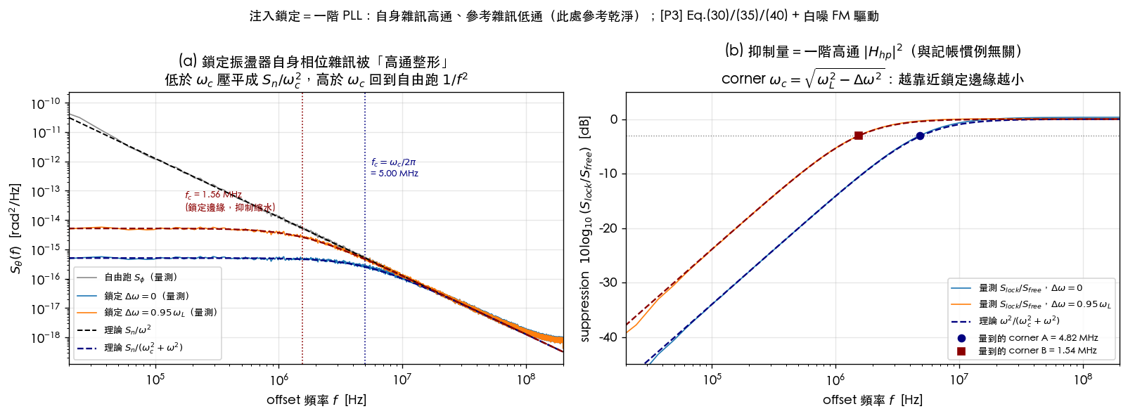
How to read this figure: (a) the gray line is free-running $1/f^2$; blue/orange are the locked $S_\theta$ — the three curves overlap at high frequency (the injection has no reach there), and are flattened into the $S_n/\omega_c^2$ plateau at low frequency; the dashed line is first-order theory, matching throughout. (b) dividing the two locked PSDs by the free-running one gives a clean first-order high-pass $\omega^2/(\omega_c^2+\omega^2)$; the $-3$ dB crossing is the corner — case B ($\Delta\omega=0.95\,\omega_L$)'s corner shrinks from 5 MHz to 1.56 MHz and the plateau rises 10 dB: the degradation at the lock edge is visible to the eye.

---

Part B — When it doesn't lock: the injection-pulling spectrum

Step 1: no steady state, only "dwell-then-slip"

When $\lvert\Delta\omega\rvert\gt\omega_L$ (discuss $\Delta\omega\gt\omega_L\gt0$),

$$\frac{d\theta}{dt}=\Delta\omega-\omega_L\sin\theta\ \ge\ \Delta\omega-\omega_L\ \gt\ 0$$

is positive everywhere: $\theta$ rises monotonically, never stopping — locking fails, but the rise is highly non-uniform:

• Slowest near $\theta=\pi/2$ ($\sin\theta=1$): $d\theta/dt=\Delta\omega-\omega_L$. The oscillator "almost locks" and dwells at the phase closest to lock (quasi-lock) — the description at [P3] Sec. V-G, p.2115–2116: spends a considerable amount of time "trying" to lock.
• Fastest near $\theta=-\pi/2$: $d\theta/dt=\Delta\omega+\omega_L$ — rapid slip, sweeping through a full revolution in one burst.

So $\theta(t)$ is a sawtooth staircase of "plateau + steep ramp" (see the simulation plot (a) below), net-sliding $2\pi$ per "beat."

Step 2: the beat frequency $\omega_b$ — derived step by step

The period of one beat is the time for $\theta$ to traverse $2\pi$. Separate variables:

$$T_b=\int_0^{T_b}dt=\int_{-\pi}^{\pi}\frac{d\theta}{\Delta\omega-\omega_L\sin\theta}.$$

Use the Weierstrass half-angle substitution $u=\tan(\theta/2)$ ($\theta:-\pi\to\pi$ corresponds to $u:-\infty\to\infty$), $\sin\theta=\dfrac{2u}{1+u^2}$, $d\theta=\dfrac{2\,du}{1+u^2}$:

$$\begin{aligned} T_b&=\int_{-\infty}^{\infty}\frac{1}{\Delta\omega-\omega_L\frac{2u}{1+u^2}}\cdot\frac{2\,du}{1+u^2} =\int_{-\infty}^{\infty}\frac{2\,du}{\Delta\omega(1+u^2)-2\omega_L u}\\[4pt] &=\int_{-\infty}^{\infty}\frac{2\,du}{\Delta\omega\,u^2-2\omega_L u+\Delta\omega} \qquad\text{(complete the square in the denominator)}\\[4pt] &=\int_{-\infty}^{\infty}\frac{2\,du}{\Delta\omega\Big(u-\frac{\omega_L}{\Delta\omega}\Big)^2+\frac{\Delta\omega^2-\omega_L^2}{\Delta\omega}} =\frac{2}{\sqrt{\Delta\omega^2-\omega_L^2}}\Big[\arctan\Big(\frac{\Delta\omega\,u-\omega_L}{\sqrt{\Delta\omega^2-\omega_L^2}}\Big)\Big]_{-\infty}^{\infty}\\[4pt] &=\frac{2}{\sqrt{\Delta\omega^2-\omega_L^2}}\cdot\pi . \end{aligned}$$

(The second-to-last step uses $\int\frac{du}{a(u-u_0)^2+c}=\frac{1}{\sqrt{ac}}\arctan\big(\sqrt{a/c}\,(u-u_0)\big)$, with $a=\Delta\omega\gt0$, $c=(\Delta\omega^2-\omega_L^2)/\Delta\omega\gt0$, and $\arctan$ spans $\pi$ over the full range.)

$$\boxed{\ \omega_b\equiv\frac{2\pi}{T_b}=\sqrt{\Delta\omega^2-\omega_L^2}\ } \qquad\text{([P4] Eq.(34), p.2130, taking }N=1\text{)}$$

The same substitution also gives the closed-form solution in the unlocked regime (equivalent to the ideal-LC special case of [P4] Eq.(33), p.2130):

$$\tan\frac{\theta(t)}{2}=\frac{\omega_L}{\Delta\omega}+\frac{\omega_b}{\Delta\omega}\tan\frac{\omega_b (t-t_0)}{2}.$$

Units: rad/s ✓ ($\Delta\omega,\omega_L$ share units, take the square root of the squared difference). Two limits:

• $\Delta\omega\gg\omega_L$: $\omega_b\to\Delta\omega$ — the sideband spacing approaches the detuning itself, the injection degenerates into a single small spur, the oscillator is essentially free-running ✓ (self-consistency check).
• $\Delta\omega\to\omega_L^+$: $\omega_b\to0$ — critical slowing down: the dwell segment stretches without bound, the beat frequency vanishes, all comb teeth collapse toward the injection frequency — this is the instant of "locking." Note it and Part A's $\omega_c=\sqrt{\omega_L^2-\Delta\omega^2}$ are two sides of the same square root: inside lock it's called the pull-in frequency, outside lock it's called the beat frequency ([P4] Eq.(32) vs Eq.(34) — a Pythagorean pair).

Numerically (lab_27 uses a 3-4-5 right triangle, verifiable by mental arithmetic): $\Delta f=100$ kHz, $f_L=60$ kHz → $f_b=\sqrt{100^2-60^2}=80$ kHz.

Step 3: spectral structure — comb spacing $\omega_b$, one edge pinned to the injection

$\theta$ nets $2\pi$ every $T_b$, so $\theta(t)=\omega_b t+p(t)$, with $p$ periodic of period $T_b$. The output voltage

$$V(t)=\cos\big(\omega_{inj}t+\theta(t)\big)$$

has an analytic signal containing $e^{j\theta}=e^{j\omega_b t}e^{jp(t)}$, and the Fourier series of $e^{jp(t)}$ has only components at $k\omega_b$ — so the spectrum is a comb of spacing $\omega_b$, with lines at

$$\omega=\omega_{inj}+k\,\omega_b,\qquad k\in\mathbb{Z},$$

where the $k=0$ line falls exactly at the injection frequency ([P4] Sec. V-B, p.2130: the tone at one edge of the spectrum always occurs right at the injection frequency). The oscillator's average frequency is $\omega_{inj}+\omega_b$ (near the $k=1$ main line), which lies between $\omega_{inj}$ and $\omega_0$: it has been "pulled" away from free-running by $\Delta\omega-\omega_b$ (lab_27 numbers: $100-80=20$ kHz) — this is exactly where the name "pulling" comes from. Detail worth noting ([P3] footnote 18, p.2116): unless $\omega_{inj}$ happens to be an integer multiple of $\omega_b$, $V(t)$ itself is not a periodic signal — pulling fundamentally destroys the oscillator's periodicity.

The interactive widget below integrates the Adler ODE right in your browser (RK2), takes an FFT of $V(t)=\cos(\omega_{inj}t+\theta(t))$, and lets you slide $r=\Delta\omega/\omega_L$ from locked into pulling with your own hands, watching the spectrum morph from "a single tone" into "a one-sided comb"; the measured $\omega_b$ is compared live against the closed form $\sqrt{\Delta\omega^2-\omega_L^2}$ derived above:

Injection-pulling spectrum explorer (RK2 Adler integration → FFT)

Δω / ω_L (r)1.50

FFT length

state

PULLING — comb

r > 1

ω_b (theory)

1.1180

√(Δω²−ω_L²)

ω_b (measured, FFT)

1.1115

error 0.59%

Reading the plot: the red dashed line is the injection frequency ω_inj. Slide r = Δω/ω_L below 1 and the spectrum collapses to a single clean line at ω_inj — the oscillator is locked onto the injection, θ(t) has settled to a constant, so V(t) = cos(ω_inj t + θ_ss) is a pure tone. Push r above 1 and a one-sided comb appears, spaced by ω_b = √(Δω²−ω_L²), with one edge line pinned exactly at ω_inj — this is the closed form derived in Part B above ([P4] Eq.(34)). The "ω_b (measured, FFT)" readout takes the median spacing between the strongest comb lines (with parabolic sub-bin interpolation) and compares it to the theoretical closed form live.

Model: RK2 (midpoint) integration of dθ/dt = Δω − ω_L·sin(θ) for 4096 steps (dt = 0.02, ω_L = 1 normalized), Hann-windowed FFT of V(t) = cos(ω_inj t + θ(t)) over the last {1024 or 2048}-point window (radix-2 Cooley–Tukey, written inline, no external deps), peak positions refined with parabolic interpolation. Offline verification (Node/Python, same algorithm): at r = 1.5 the measured comb spacing matches √(Δω²−ω_L²) to within ≈0.1% using the 2048-point FFT — see the write-up in Part B and lab_27 for the reference numbers.

Step 4: why is it "one-sided"?

Physical argument. The instantaneous frequency is

$$\omega_{osc}(t)=\omega_{inj}+\frac{d\theta}{dt}\in[\,\omega_{inj}+\Delta\omega-\omega_L,\ \omega_{inj}+\Delta\omega+\omega_L\,],$$

and the entire range sits on the same side of the injection ($\Delta\omega\gt\omega_L$ guarantees a positive lower bound). And the time-weighting is extremely skewed: $\theta$ dwells longest in the dwell segment ($\omega_{osc}\approx\omega_{inj}+\Delta\omega-\omega_L$, closest to the injection), while the slip segment flashes by — so spectral energy piles up on "the side of the injection frequency toward $\omega_0$," hugging the injection and decaying outward; the other side of the injection is nearly empty. This contrasts sharply with symmetric FM (sinusoidal phase modulation → symmetric Bessel sidebands): the phase-modulating waveform of pulling is a sawtooth, not a sinusoid.

Rigorous argument (advanced, one paragraph). Let $z=e^{j\theta}$; the Adler equation becomes the Riccati equation $\dot z=j\Delta\omega\,z-\tfrac{\omega_L}{2}(z^2-1)$. The Riccati solution is a Möbius (fractional-linear) transform of coefficients, letting us write the periodic solution as $z=\dfrac{c+d\,w}{1+b\,w}$ ($w=e^{j\omega_b t}$, $\lvert b\rvert\lt1$); expanding the geometric series $\dfrac{1}{1+bw}=\sum_k(-b)^k w^k$ leaves only powers $k\ge0$ — so in this idealized Adler model the comb is strictly one-sided, and the amplitudes decay geometrically, with ratio

$$r=\frac{\omega_L}{\Delta\omega+\omega_b}$$

(power drops by $r^2$ per line). This closed-form spectrum is a standard result (external literature, not among the five source PDFs: Armand 1969, see the end of this page); the rest of this page verifies it numerically with simulation. lab_27's 3-4-5 parameters: $r=60/(100+80)=1/3$, i.e. $20\log_{10}3=9.54$ dB per line.

lab_27: integrating the unlocked Adler ODE → FFT

Model: RK4 integration of $d\theta/dt=\Delta\omega-\omega_L\sin\theta$ (deterministic; noise turned off to isolate the pulling comb itself), building $V(t)=\cos(\omega_{inj}t+\theta(t))$, then a Hann-windowed FFT.

Parameter	Value	Unit	Note
$f_{inj}$	1.000	MHz	injection frequency (toy scale — the Adler equation is already the averaged slow dynamic)
$f_0$	1.100	MHz	free-running frequency ($\Delta f=+100$ kHz)
$f_L$	60	kHz	half lock range ($\Delta f\gt f_L$ → fails to lock)
$f_b$ (theory)	80.000	kHz	$\sqrt{100^2-60^2}$ (3-4-5)
$f_s$, length	16 MHz, $2^{21}$ points	—	131 ms ≈ 10486 beats, FFT resolution 7.6 Hz

Core code (full script: simulations/lab_27_pulling_spectrum.py):

def rhs(th):                                   # unlocked Adler ([P3] Eq.(30) sinusoidal reduction)
    return DW - OMEGA_L*np.sin(th)             # [rad/s]
# ... RK4 integration to get theta[k] ...
V    = np.cos(OMEGA_INJ*t + theta)             # the pulled output voltage
spec = np.abs(np.fft.rfft(V*np.hanning(V.size)))**2

Verified output numbers (PYTHONPATH=. python3 simulations/lab_27_pulling_spectrum.py):

print(f_b_from_slope)                 # -> 79.999 kHz from ⟨dθ/dt⟩, theory 80.000 -> ratio 1.0000
print(f_b_from_fft)                   # -> 80.000 kHz from spectral comb spacing -> ratio 1.0000
print(step_k1_k2, step_k2_k3)         # -> -9.54 dB, -9.54 dB adjacent comb-line power step (theory 20log10(3)=-9.54)
print(mirror_side)                    # -> -194.1 dB f_inj-f_b vs f_inj+f_b: mirror side = numerical zero (strictly one-sided)
print(edge_tone)                      # -> -8.52 dB the edge line at the injection frequency relative to the k=+1 main line
print(pulled_by)                      # -> 20.0 kHz average frequency 1.080 MHz, pulled away from f_0=1.100 MHz

Main spectral lines (relative to the strongest line): 1.080 MHz (0 dB, $k{=}1$), 1.000 MHz ($-8.2$ dB, $k{=}0$ = injection), 1.160 ($-10.5$), 1.240 ($-19.2$), 1.320 ($-28.3$), 1.400 MHz ($-38.1$ dB) — from $k\ge2$ onward each line drops exactly 9.54 dB, matching the geometric ratio $r^2=(1/3)^2$ to the digit.

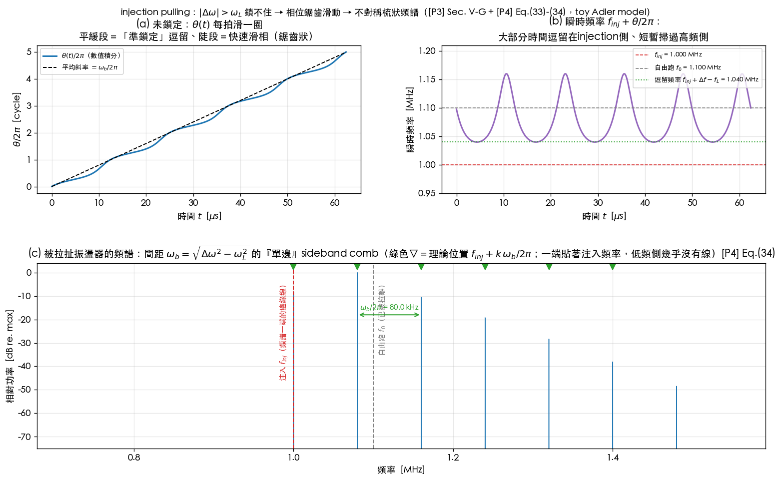
How to read this figure: (a) $\theta/2\pi$ climbs one step per beat, the flat segments are the quasi-lock dwell; (b) the instantaneous frequency spends most of its time pinned near 1.04 MHz ($f_{inj}+\Delta f-f_L$, the "dwell frequency" closest to injection), with brief excursions to 1.16 MHz; (c) spectrum: the red dashed line = injection at 1.000 MHz (the comb's edge), the gray dashed line = free-running at 1.100 MHz (no line there anymore — it's been pulled away), green ▽ = theoretical positions $f_{inj}+k\,f_b$; the injection's left side is completely clean — the one-sided comb is the clearest fingerprint of pulling.

---

Injection waveform design: the ceiling on the lock range ([P3] Sec. VI, Cauchy–Schwarz)

One of Part A's conclusions is that $\omega_L$ is not just "the range within which you can lock" — it is also the ceiling on the noise-suppression bandwidth ($\omega_c\le\omega_L$). So "for the same injection power, how far can $\omega_L$ be pushed" is a real-money design question. [P3] Sec. VI (pp. 2119–2120) gives an answer clean enough to memorize; this section re-derives it step by step, following the paper, and verifies it numerically on three ISFs.

Physical intuition (conclusion first): the ISF is the dashboard showing "how persuadable the oscillator is right now." A fixed current budget should be spent entirely at the phases where $\lvert\tilde\Gamma\rvert$ is large (where the node voltage transitions are steepest and the phase is easiest to push), and not a cent at the phases where $\tilde\Gamma\approx0$. A sinusoidal injection cannot do this — it is forced to spread its money uniformly across the whole period. The optimum is to "shape the injection waveform like the ISF itself" ([P3] Fig. 18, p.2118's concept cartoon).

Step 0: define "how big" the injection is — why rms?

To compare waveforms of different shapes, you first need a common measuring stick for "equally big." A multi-harmonic waveform has no unique "amplitude," so [P3] uses the rms injection current ([P3] Eq.(43), p.2119, verbatim):

$$I_{rms}\equiv\sqrt{\langle i_{inj}^2\rangle}:=\sqrt{\frac{1}{T_{inj}}\int_{T_{inj}}i_{inj}(t)^2\,dt}\ .$$

Units: $\sqrt{\text{A}^2}=\text{A}$ ✓. Why is rms the right proxy for "power"? [P3] p.2119 + Fig. 17: a practical injection circuit is usually a differential pair commutating a static tail current $I_{bias}$; the instantaneous $\lvert i_{inj}\rvert$ is capped by the tail current, so $I_{rms}\le I_{bias}$, and the injection circuit's average power consumption is at least $I_{rms}V_{DD}$ — fixing $I_{rms}$ ≈ fixing the floor of the injection circuit's power, and it is well-defined for any waveform.

The three-step derivation: inner product → Cauchy–Schwarz → equality condition

Step 1: the lock range is the extremum of an inner product. The starting point is again the verified lock characteristic ([P3] Eq.(33), p.2114):

$$\Omega(\theta)=\frac{1}{T_{inj}}\int_{T_{inj}}\tilde\Gamma(\omega_{inj}t+\theta)\,i_{inj}(t)\,dt .$$

At fixed $\theta$ this is precisely the time-averaged inner product of two periodic signals, $\langle u,v\rangle=\frac{1}{T}\int_T uv\,dt$, with $u_\theta(t)=\tilde\Gamma(\omega_{inj}t+\theta)$ [rad/C] and $v(t)=i_{inj}(t)$ [A]. The lock condition (the generalization of Part A's Step 1; the steady state of [P3] Eq.(38)) is that $\Delta\omega$ falls within the range of $\Omega$: the upper/lower lock edges are $\max_\theta\Omega$ and $\min_\theta\Omega$. So "make the lock range big" = "make the extrema of this inner product big" — the circuit problem has become a functional inequality.

Step 2: the Cauchy–Schwarz bound. For every $\theta$ and every waveform (the integral form of Cauchy–Schwarz: $\lvert\langle u,v\rangle\rvert\le\lVert u\rVert\,\lVert v\rVert$):

$$\lvert\Omega(\theta)\rvert\;\le\;\underbrace{\sqrt{\tfrac{1}{T_{inj}}\!\int_{T_{inj}}\!\tilde\Gamma^2(\omega_{inj}t+\theta)\,dt}}_{=\ \tilde\Gamma_{rms}\ \text{(independent of }\theta\text{)}}\cdot\underbrace{\sqrt{\tfrac{1}{T_{inj}}\!\int_{T_{inj}}\!i_{inj}^2(t)\,dt}}_{=\ I_{rms}\ \text{(Eq.(43))}}$$

The first factor is independent of $\theta$: one injection period sweeps the entire $2\pi$ of $\tilde\Gamma$ exactly once, and a mean square does not care at which phase the sweep starts. Units: $\text{rad/C}\times\text{A}=\text{rad/s}$ ✓. Therefore, no matter what shape you give the waveform, the lock range can never exceed ([P3] Eq.(45), p.2120, verbatim)

$$\omega_L^*=I_{rms}\tilde\Gamma_{rms}\ .$$

Step 3: the equality condition — the waveform = the shape of the ISF. Cauchy–Schwarz holds with equality ⟺ the two "vectors" are parallel: $i_{inj}(t)=\lambda\,\tilde\Gamma(\omega_{inj}t+\text{const})$. Normalizing the size of $\lambda$ to the given $I_{rms}$ via Eq.(43) gives the optimal injection waveform ([P3] Eq.(44), p.2119, verbatim; $x=\omega_{inj}t$ is the linear injection phase):

$$i_{inj,0}^{*}(x)=\pm\frac{I_{rms}}{\tilde\Gamma_{rms}}\,\tilde\Gamma(x)\ .$$

Three key points:

• With the + sign, $\Omega(\theta)$ becomes the ISF's autocorrelation $\times\,I_{rms}/\tilde\Gamma_{rms}$, reaching $+I_{rms}\tilde\Gamma_{rms}$ at the aligned point — optimizing the upper lock edge; the − sign likewise optimizes the lower edge ([P3] p.2120 states it explicitly: the positive solution for the upper edge, the negative for the lower). One waveform cannot push both edges to the ceiling simultaneously — see the numbers in Check 2 below.
• No manual alignment needed: $\theta$ is the oscillator's own degree of freedom; the locking mechanism adjusts it onto the stable branch satisfying $\Delta\omega=\Omega(\theta)$. Waveform design only needs the shape right — the phase is found by the physics itself.
• Factor bookkeeping: Eq.(45) contains no 2 and no 4 — both sides are rms quantities. The $\tfrac12$ in the classical sinusoidal result $\omega_L=\tfrac12 I_{inj}\lvert\tilde\Gamma_1\rvert$ ([P3] Eq.(35)) is the projection integral $\langle\cos^2\rangle=\tfrac12$, with $I_{inj}$ a peak value; rewritten in rms ($I_{rms}=I_{inj}/\sqrt2$) it reads $\omega_{L,sine}=I_{rms}\lvert\tilde\Gamma_1\rvert/\sqrt2$. All of these $\sqrt2$'s and $2$'s are peak↔rms conversions and projection constants — nothing to do with the SSB $/2$, $/4$ bookkeeping conventions.

Check 1: pure-sine ISF — a sinusoidal injection is "already" optimal (the ratio must be 1)

The ideal LC's $\tilde\Gamma(x)=-\sin(x)/q_{max}$ is itself a single-tone sinusoid, so the waveform "shaped like the ISF" is a sine — the theorem predicts a sinusoidal injection already sits at the ceiling. Compute both sides (the true-LC $\Gamma_{rms}=1/\sqrt2$ branch, not the representative value 0.5):

$$\omega_{L,sine}=\frac{I_{rms}\lvert\tilde\Gamma_1\rvert}{\sqrt2}=\frac{I_{rms}}{\sqrt2\,q_{max}},\qquad \omega_L^*=I_{rms}\tilde\Gamma_{rms}=\frac{I_{rms}}{\sqrt2\,q_{max}}\quad\Rightarrow\quad\text{ratio}=1 .$$

Numbers (reusing Part A's canonical case: $q_{max}=1$ pC, peak $62.83\ \mu$A i.e. $I_{rms}=44.43\ \mu$A): $\omega_L^*=4.443\times10^{-5}\times0.7071/10^{-12}=3.14\times10^7$ rad/s → $f_L^*=5.000$ MHz, identical to Part A's sinusoidal lock range. Dimension check: A × rad/C = (C/s)(rad/C) = rad/s ✓. (The simulation prints f_L sine = 5.0000 MHz, f_L matched = 5.0000 MHz, gain = 1.0000.)

Teaching point: this is no coincidence — it is forced by "the ISF has only one harmonic." The only thing a sinusoidal injection can buy is $\tilde\Gamma_1$, and a pure-sine ISF keeps all of its rms in $\tilde\Gamma_1$. For waveform design to "make money," the ISF must hide energy where a sine cannot reach: DC ($c_0$) or higher harmonics. The next two checks demonstrate one of each.

Check 2: asymmetric toy ISF — matched injection profits at DC (and only on one edge)

The site toy $\Gamma(\theta)=\cos\theta+0.3$ ($\alpha=0.3$, DC value $c_0/2=0.3$): $\Gamma_{rms}=\sqrt{\alpha^2+\tfrac12}=0.7681$, $c_1=1$. Closed-form gain:

$$G=\frac{\omega_L^*}{\omega_{L,sine}}=\frac{I_{rms}\Gamma_{rms}/q_{max}}{I_{rms}\,c_1/(\sqrt2\,q_{max})}=\frac{\sqrt2\,\Gamma_{rms}}{c_1}=\sqrt{1+2\alpha^2}=1.0863 .$$

(Simulation: gain = 1.0863, $f_L$ from 5.0000 → 5.4314 MHz.) The matched waveform is just the shape of $\cos+\alpha$ — the extra DC share of the current couples to the ISF's $c_0$, something a zero-mean sine can never buy. But note the one-sidedness (the $\pm$ choice): in units of $I_{rms}/q_{max}$, the simulation prints matched(+) upper/lower edges $=+0.7681$/$-0.5338$, versus the sine's $\pm0.7071$ — the upper edge gains 8.6% while the lower edge loses 24%; for the lower edge, switch to the $-$ sign. The DC injection shifts the whole lock characteristic upward — exactly the mechanism by which "the upper and lower lock edges can have the same sign," as the caption of [P3] Fig. 10 notes.

Check 3: ring-style narrow-pulse ISF — gain $\approx\sqrt{\eta N/3}$, ≈ ×2 at 17 stages

A ring's ISF energy concentrates at the transitions. As a toy, use the [P2] App.B triangular-pulse construction ($A=1$, symmetric rise/fall): two opposite-sign triangular pulses, height $h=1/f'$, half-width $w=1/f'$ rad, with $f'=\eta N/\pi$ (from [P2] Eq.(54), p.803 with $A=1$). Sanity check: this construction's $\Gamma_{rms}$ lands exactly back on [P2] Eq.(55) ($A=1$): the simulation prints 0.05634 = the closed form $\sqrt{2\pi^2/3\eta^3}/N^{1.5}=$ 0.05634 ✓.

The narrow-pulse closed-form gain (three lines): a single pulse of area $hw$ gives $c_1\approx 2hw/\pi$ (the two opposite-sign pulses sit $\pi$ apart, so their projections onto $\sin$ add with the same sign); $\Gamma_{rms}^2=\tfrac{1}{2\pi}\cdot2\cdot\tfrac23h^2w=\tfrac{2h^2w}{3\pi}$; substituting $h=w=1/f'$, $f'=\eta N/\pi$:

$$G=\frac{\sqrt2\,\Gamma_{rms}}{c_1}\approx\sqrt{\frac{2\cdot\frac{2h^2w}{3\pi}}{\frac{4h^2w^2}{\pi^2}}}=\sqrt{\frac{\pi}{3w}}=\sqrt{\frac{\eta N}{3}}\ .$$

$N=17$, $\eta=0.75$: $G=\sqrt{4.25}=2.0616$ (full numerical simulation 2.0720; the 0.5% difference is the $\mathrm{sinc}^2$ correction for the pulses' finite width). With units attached: for the same $I_{rms}=44.43\ \mu$A and $q_{max}=1$ pC, sine 192.3 kHz → matched 398.4 kHz.

This ×2 is not the toy congratulating itself: [P3] Fig. 19 (p.2119) runs transistor-level simulations of a 17-stage single-ended ring — injecting pulses shaped close to the ISF (Fig. 19(b), not a strict ISF replica), and p.2120 states verbatim: "the lock range is almost doubled compared to a sinusoidal injection of the same power." The toy's $\sqrt{\eta N/3}\approx2.06$ agrees with the real circuit's "almost doubled" at the level of the factor 2, not the decimals (the real ISF's details differ). The gain is $\propto\sqrt N$: more stages → transitions occupy a smaller fraction of the phase → the sine wastes more — long rings are where waveform design pays off the most.

An honest toy footnote: the site's cruder gamma_triangular toy is $\pi$-periodic (the rising and falling triangles repeat perfectly symmetrically), so it has even harmonics only — the simulation prints its $c_1=0.000000$, $c_2=0.3625$: a fundamental-frequency sine cannot lock it at all (effectively only superharmonic injection would work). This is a toy artifact (a real ring's rising and falling edges are never so symmetric that only even harmonics survive), but it demonstrates the same lesson in the most extreme way: a sine can only buy $c_1$; if the ISF puts no energy in $c_1$, the money is wasted.

lab_33: numerical verification + figure

Model: on a 4096-point phase grid, write the periodic average of [P3] Eq.(33) as a circular correlation; for each of the three ISFs compute the lock characteristic under a sinusoidal and a matched injection (same $I_{rms}$); the extrema are the lock edges.

Core code (full script: simulations/lab_39_optimal_injection.py):

def lock_characteristic(gt, i_wave):                  # [P3] Eq.(33): circular correlation
    Gf, If = np.fft.rfft(gt), np.fft.rfft(i_wave)
    return np.fft.irfft(np.conj(If) * Gf, gt.size) / gt.size   # Ω(θ) [rad/s]

i_sine = np.sqrt(2)*I_RMS*np.cos(X)                   # sine of the same I_rms
i_star = (I_RMS/gt_rms) * gt_p                        # [P3] Eq.(44), + sign
wl_sine = lock_characteristic(gt_p, i_sine).max()     # upper lock edge [rad/s]
wl_star = lock_characteristic(gt_p, i_star).max()     # should touch I_rms·Γ̃_rms

Verified output numbers (PYTHONPATH=. python3 simulations/lab_39_optimal_injection.py):

print(fL_sine_LC, fL_matched_LC)      # -> 5.0000 MHz, 5.0000 MHz pure-sine ISF: sine already optimal (gain = 1.0000)
print(gain_asym)                      # -> 1.0863 cos+0.3 matched gain = analytic sqrt(1+2α²)=1.0863
print(edges_asym)                     # -> +0.7681/-0.5338 matched(+) upper/lower edges (units of I_rms/q_max; sine ±0.7071)
print(gamma_rms_ring)                 # -> 0.05634 = [P2] Eq.(55) closed form 0.05634 (construction sanity check)
print(fL_sine_ring, fL_matched_ring)  # -> 0.1923 MHz, 0.3984 MHz N=17 ring toy, same I_rms=44.43 μA
print(gain_ring)                      # -> 2.0720 closed form sqrt(ηN/3)=2.0616 (0.5% difference = sinc² correction)
print(matched_over_bound)             # -> 1.0000 the matched injection exactly touches the Cauchy–Schwarz bound (all three cases)
print(c1_site_triangular)             # -> 0.000000 the site toy gamma_triangular is π-periodic: a fundamental sine cannot lock it (artifact)

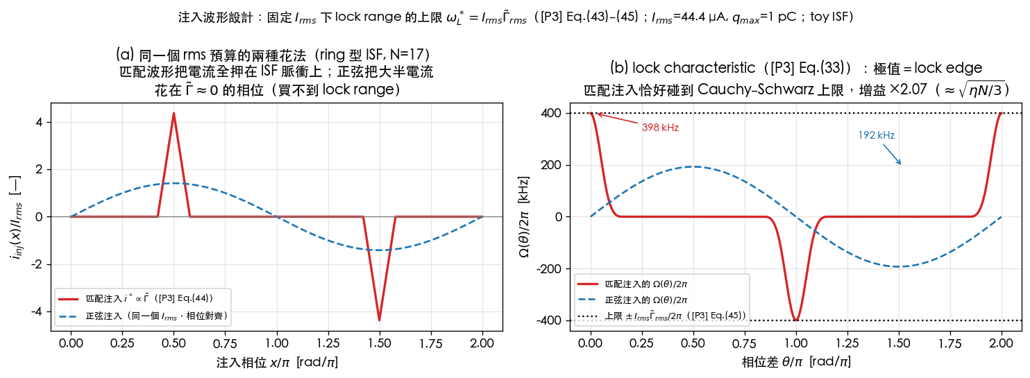
How to read this figure: (a) the two waveforms have exactly the same rms (both 44.43 μA); the only difference is where the money goes — the matched injection (red) concentrates the current into narrow pulses shaped like the ISF, while the sine (blue dashed) spends most of its current in the dead zone where $\tilde\Gamma\approx0$; (b) the corresponding lock characteristics: the extrema are the lock edges, and the red curve exactly touches the dotted theoretical bound $\pm I_{rms}\tilde\Gamma_{rms}/2\pi=\pm398$ kHz, while the sine only reaches 192 kHz — the same power, ×2.07 the lock range (and Part A's noise-suppression-bandwidth ceiling $\omega_c\le\omega_L$ scales by ×2.07 along with it).

Conditions for validity and failure modes (this section)

Condition	When it holds	What happens when it fails
Weak-injection linearity ([P3] Eq.(36)–(37): $I_{inj}\ll I_{max}=\omega_0 q_{max}$)	Eq.(33) linear in $i_{inj}$; the Cauchy–Schwarz argument holds	Strong injection: $\Omega$ departs from the linear prediction; [P3] Fig. 19's simulations use $I_{rms}$ beyond $I_{max}=0.72$ mA and still roughly agree (the Sec. V-H observation)
"Size" measured by $I_{rms}$ (Eq.(43))	Optimum = Eq.(44), ceiling = Eq.(45)	Change the constraint and the optimum changes: if the peak current is limited, $\lvert i_{inj}\rvert\le I_{pk}$, the optimum becomes the square-like $i=I_{pk}\,\mathrm{sign}(\tilde\Gamma)$ with ceiling $I_{pk}\langle\lvert\tilde\Gamma\rvert\rangle$ (this site's extension, not in [P3])
The injector can generate the waveform	Full $G$ collected	Narrow pulses need bandwidth up to $\sim N$ harmonics: at $f_0=5$ GHz, a 17-stage pulse needs spectral content out to ~85 GHz — in practice the pulses are widened and $G$ degrades smoothly along the ISF autocorrelation (no cliff)
ISF known and stable	Waveform can be designed offline	The ISF must come from simulation ([P3] Sec. V-H's impulse-response method) or closed forms ([P2] App.B); when PVT drifts the ISF, $G$ is discounted, but the locked phase $\theta_{ss}$ re-aligns automatically
The goal is the maximum lock range	All of this section	Sometimes you want to minimize it (multiple oscillators interfering, reducing coupling) — the same framework run in reverse ([P3] p.2120 closing explicitly flags this direction)

Three design sentences: (i) for LC (near-sine ISF), don't bother — a sinusoidal injection is already at the ceiling (exactly gain 1.0000 for a pure sine; the residual gain for near-sine ISFs is second-order small); (ii) ring/relaxation (pulse-type ISFs) benefit the most from waveform design, with gain $\approx\sqrt{\eta N/3}$ growing as the square root of the stage count; (iii) this gain simultaneously scales Part A's $\omega_c$ — at the same power the noise-suppression-bandwidth ceiling also gains ×G, which is the number SerDes ILO deskew actually cares about.

---

Design knobs (rolling both parts into an actionable checklist)

1. Push $\Delta\omega$ to the center of the lock range: the noise-suppression bandwidth $\omega_c=\sqrt{\omega_L^2-\Delta\omega^2}$ is only maximal at $\Delta\omega=0$. The goal of a calibration/tuning loop is not just "get locked," it's "get locked in the middle."
2. Two ways to increase $\omega_L$ ([P3] Eq.(35): $\omega_L=\tfrac12 I_{inj}\lvert\tilde\Gamma_1\rvert$): raise the injection current (at the cost of power and spurs), or use waveform design to align injection harmonics with ISF harmonics ([P3] Sec. VI's injection waveform design — effectively a free boost to $\omega_L$ and $\omega_c$; for the quantitative ceiling and the optimal waveform see the "Injection waveform design" section above: $\omega_L^*=I_{rms}\tilde\Gamma_{rms}$, with gain $\approx\sqrt{\eta N/3}$ for ring-type ISFs). Ceiling to watch: $I_{inj}\ll I_{max}=\omega_0 q_{max}$ ([P3] Eq.(36)–(37)).
3. Leave edge margin: the plateau penalty is $1/\cos^2\theta_{ss}$. $\lvert\Delta\omega\rvert/\omega_L=0.5$ only costs $+1.2$ dB; $0.95$ costs $+10.1$ dB. Budget for PVT drift should be counted against $\Delta\omega/\omega_L$.
4. Recognize the fingerprint of pulling: a comb next to the carrier that is one-sided, evenly spaced by $\omega_b$, with one edge pinned exactly at some fixed frequency → that fixed frequency is the aggressor's frequency. Countermeasures, in order: add isolation (layout, guard ring, supply/substrate filtering); move the frequency plan (pull $\Delta\omega$ larger, so the comb spacing $\omega_b\to\Delta\omega$ moves further out and the amplitude $r\to0$ shrinks); or, conversely, just lock onto it deliberately (make $\omega_L$ larger than $\lvert\Delta\omega\rvert$, so the spur comb collapses into a clean locked carrier). The most dangerous case is neither near nor far: when $\Delta\omega$ is only slightly above $\omega_L$, $\omega_b$ is tiny, the spur sits right next to the carrier (in-band, can't be filtered out) and $r\to1$ (slow decay, a dense, tall comb).
5. Connection to SerDes: injection-locked clock distribution (forwarded-clock / multi-lane ILO deskew) is using $\omega_c$ as the jitter tracking bandwidth — reference jitter below $\omega_c$ is copied through (a benefit for lanes with common jitter: shared source, correlated cancellation), while above $\omega_c$ cleanliness relies on the local oscillator itself (the same old homework of $q_{max}$, $\Gamma_{rms}$, design_tradeoffs). The trade-off structure is exactly isomorphic to a CDR: see serdes_clocking_connection, lab_13.

Conditions for validity and failure modes

Condition	When it holds	What happens when it fails
Weak injection $I_{inj}\ll I_{max}=\omega_0q_{max}$ ([P3] Eq.(36)–(37), p.2115)	Generalized Adler / lock characteristic linear in $i_{inj}$	Strong injection: prediction error of $\Omega(\theta)$ grows (though [P3] Sec. V-H simulations show $I_{inj}\sim I_{max}$ is still roughly usable)
$\theta$ slowly varying (near-constant over one period)	Time-synchronous averaging (Eq.(30)) holds	Detuning too large, or $\omega_b$ close to $\omega_{inj}$: the averaging breaks down
Sinusoidal injection + ideal-LC ISF	This page's closed form $-\omega_L\sin\theta$	Arbitrary waveform/topology: fall back to the general $\Omega(\theta)$; the corner generalizes to $\omega_c=-\Omega'(\theta_{ss})$ ([P3] Eq.(40)), and the geometric ratio of the one-sided comb no longer has a simple closed form
Small noise, $\lvert\Delta\omega\rvert$ well clear of the edge	Linearization (OU) holds, $S_\theta=S_n/(\omega_c^2+\omega^2)$	Near the edge: the potential well shallows → cycle slips → the spectrum grows pulling-like residual spurs, the OU formula fails
Amplitude dynamics ignored	Pure-phase model (this entire page)	Strong-injection LC: needs [P4]'s APF/AM correction (paper_004); [P4] Fig. 14(c) shows adding APF substantially improves accuracy of the pulled spectrum
The noise-shaping derivation itself	Standard injection-locking noise theory	Not in the five source PDFs (Kurokawa 1973; [P4] points to [29, Ch. 7]); this page derives it from scratch and cross-checks with simulation

Key takeaways

• Injection locking = a first-order PLL: linearizing [P3]'s generalized Adler gives $d(\delta\theta)/dt=-\omega_c\delta\theta+n$, loop bandwidth $\omega_c=\omega_L\cos\theta_{ss}=\sqrt{\omega_L^2-\Delta\omega^2}$ — exactly the pull-in frequency of [P3] Eq.(40) (general topology: $\omega_c=-\Omega'(\theta_{ss})$).
• Self-noise is high-passed, reference noise is low-passed, sharing the corner $\omega_c\le\omega_L$; under a white FM drive, $S_\theta=S_n/(\omega_c^2+\omega^2)$, low-frequency plateau $S_n/\omega_c^2$, finite total variance $S_n/(4\omega_c)$ (simulation: corner and plateau both match theory to within 0.96-1.00×).
• Suppression vanishes at the lock edge: as $\Delta\omega\to\omega_L$, $\cos\theta_{ss}\to0$, the plateau rises as $1/\cos^2\theta_{ss}$ ($+10.1$ dB at $0.95\,\omega_L$) — locked doesn't mean clean; margin must be budgeted.
• When it doesn't lock: $\theta$ slides in a sawtooth (dwell + slip), beat frequency $\omega_b=\sqrt{\Delta\omega^2-\omega_L^2}$ (derived step by step; [P4] Eq.(34)); the spectrum is a one-sided comb: lines at $\omega_{inj}+k\omega_b$, one edge exactly at the injection frequency ([P4] Sec. V-B), amplitude decaying geometrically as $r=\omega_L/(\Delta\omega+\omega_b)$ (external, Armand 1969; simulation matches $-9.54$ dB/line to the digit).
• Two faces of the same square root: inside lock, $\sqrt{\omega_L^2-\Delta\omega^2}$ = the noise-suppression corner; outside lock, $\sqrt{\Delta\omega^2-\omega_L^2}$ = the spur comb spacing. In design, you want one of them large (wide suppression) and the other either large or zero (spur far away, or locked out entirely).
• The ceiling of waveform design: at fixed $I_{rms}$ (= the proxy for injection power, [P3] Eq.(43)), the Cauchy–Schwarz ceiling of the lock range is $\omega_L^*=I_{rms}\tilde\Gamma_{rms}$ ([P3] Eq.(45)), with equality ⟺ $i_{inj}\propto\tilde\Gamma$ (Eq.(44), the $\pm$ selecting the upper/lower edge). Pure-sine ISF: a sine is already optimal (gain = 1.0000); ring-type pulse ISF: $G\approx\sqrt{\eta N/3}$, ×2.07 at $N=17$ — the same order as [P3] Fig. 19's "almost doubled."

Further reading

• lab_36_lock_acquisition (v8): lock-acquisition transients, critical slowing, and noise-induced cycle slips (SDE experiments).

• Source and verification of the generalized Adler and lock characteristic: paper_003 ([P3] Eq.(26)/(30)/(33)/(35)/(38)–(40))

• Original source of the optimal injection waveform and the rms constraint: [P3] Sec. VI, Eq.(43)–(45), pp.2119–2120 (Fig. 17: rms = power proxy; Fig. 18: concept cartoon; Fig. 19: the ×2 demonstration on a 17-stage ring); triangular-pulse ring-ISF construction: [P2] App.B Eq.(52)–(55), p.803

• Original source of the closed-form beat frequency and pulled spectrum (with APF correction): paper_004 ([P4] Eq.(31)–(34), p.2130; Fig. 14)

• Mutual injection = two coupled Adler equations (QVCO's $90^\circ$ and 3 dB bookkeeping): quadrature_and_coupled_oscillators

• The same story in a second-order-loop version (reference low-pass / VCO high-pass, optimal bandwidth): pll_noise_budget, lab_13

• The "other cure" for a free-running oscillator near the carrier (Lorentzian linewidth): lorentzian_linewidth

• Source of the white FM drive $S_n=\Gamma_{rms}^2S_i/q_{max}^2$: white_noise_to_phase_noise

• The discrete-time version of subharmonic (×N) injection — the same $\omega_c$ recast as a realignment factor $\beta$, the discrete-time cousin of "locked oscillator = first-order PLL": subharmonic_injection

• The other half of the duality — the full derivation of M:N division (ILFD): injection_locked_division

• Exact large-injection transients, the APF-driven amplitude transient, and the large-injection pulling spectrum: paper_004_large_injection_transient

External literature (not among the five downloaded source PDFs)

• [E-Adler] R. Adler, "A Study of Locking Phenomena in Oscillators," Proc. IRE, vol. 34, no. 6, pp. 351–357, Jun. 1946. (The original paper on the classical Adler equation and the beat phenomenon.)
• [E-Kurokawa] K. Kurokawa, "Injection Locking of Microwave Solid-State Oscillators," Proc. IEEE, vol. 61, no. 10, pp. 1386–1410, Oct. 1973. (Noise shaping of injection-locked oscillators — the classic source for this page's Part A high-pass/low-pass result.)
• [E-Armand] M. Armand, "On the Output Spectrum of Unlocked Driven Oscillators," Proc. IEEE, vol. 57, no. 5, pp. 798–799, May 1969. (Closed-form one-sided geometric comb spectrum of an unlocked driven oscillator — this page's Part B $r=\omega_L/(\Delta\omega+\omega_b)$.)
• [E-Razavi04] B. Razavi, "A Study of Injection Locking and Pulling in Oscillators," IEEE J. Solid-State Circuits, vol. 39, no. 9, pp. 1415–1424, Sep. 2004. (An accessible modern derivation and picture of the pulled spectrum; complements the ISF generalization of [P3]/[P4].)
• Also: [P4] p.2130 points the noise analysis of locked/free-running oscillators to its own reference [29, Ch. 7] (B. Hong's PhD thesis).