β: This English translation is in beta — the Traditional-Chinese original is the authoritative version.

Subharmonic Injection: From the Impulse Train to ×N Multiplication (ILCM / ILFM)

Prerequisites: paper_003 ([P3] Sec. IV impulse train, Eq.(19)–(23), generalized Adler), paper_004 (the M:N time-synchronous average of [P4] Eq.(28)–(30)), injection_locked_division (the other half of the duality: division rides on the ISF's $N$-th harmonic), injection_locking_noise (a locked oscillator is a first-order PLL, corner $=-\Omega'(\theta_{ss})$) | Next: lab_40_subharmonic_injection (independent simulation), sampling_pll, clock_chain_budget

What this page answers:

1. Fire $f_{ref}$ pulses into an oscillator running at $f_0=N f_{ref}$ — why does it lock? On whose harmonics? Why can a pure sinusoid at $f_0/N$ not lock?
2. Why is the lock range $\propto 1/N$? How do the two routes — the [P4] Fourier average and the [P3] impulse-train arithmetic — agree term by term?
3. How much phase does each pulse "pull back" — what is the realignment factor $\beta$, what sets it, how large may it be, how many pulses to settle?
4. How is the phase noise of the locked output budgeted: reference $\times N^2$, own noise shaped by a first-order discrete-time loop, closed-form output jitter, where the reference spur comes from?
5. Design knobs: pulse width, ring vs LC, $N$, $\beta$; how does an ILCM compare with a classic PLL and a sub-sampling PLL?

Physical intuition (conclusion first): an injection-locked clock multiplier (ILCM) is not a "multiplier circuit" — it is an oscillator that already runs at $f_0\approx N f_{ref}$ and gets kicked by a reference pulse once every $N$ of its own periods. One kick = one ISF phase step $\Delta\phi=\tilde\Gamma(\theta)\,q_{inj}$; between pulses the oscillator free-runs, its phase drifts with the detuning and random-walks with noise. Locking = each kick exactly repays the phase owed over those $N$ periods; noise suppression = each kick pulls the accumulated random phase back by a fraction $\beta$. What makes the lock possible is the injection waveform's own $N$-th harmonic (the oscillator's ISF fundamental only hears things near $f_0$) — the mirror image of the divider (ILFD): division rides on ISF harmonics, multiplication on injection harmonics.

Scope of this page: advanced design page. The text, equations and footnotes of [P3] Sec. IV (p.2112) and [P4] Sec. IV (p.2129) were re-read from the enlarged PDF pages word by word (Section 0). [P4] writes out the closed form Eq.(30) only for the superharmonic case ($M=1$, a sinusoid at $N\omega_{osc}$); for the subharmonic (multiplier) side the paper gives only the general statement and footnote 10 — this page derives the multiplier closed form from Eq.(29) step by step, derives the $1/N$ law and the realignment factor from the discrete arithmetic of [P3] Sec. IV, and reconciles the two routes. Section 4, "putting noise into the discrete loop", is the textbook-level ILCM / realignment result (external literature, not in the site's 5 PDFs; two verified classics are listed at the end), derived here and checked term by term against this page's own Monte-Carlo. Every model is a phase-only, weak-injection pedagogical toy.

---

0. What the papers say — and do not say (verbatim check of [P3] p.2112 and [P4] p.2129)

0.1 [P3] Sec. IV "Locking to an Impulse Train" (p.2112)

paper_003 already teaches this section step by step: an ideal parallel LC fed by a train of current impulses of period $T_{inj}\equiv2\pi/\omega_{inj}$, each dumping a fixed charge $q_{inj}$ (Fig. 3(a); the paper takes $q_{inj}\ge0$ by convention, with the sign selecting Fig. 3(b) speed-up or Fig. 3(c) slow-down; the state-space impulse arrows in the figure are deliberately enlarged, not to scale). Four core equations:

$$\Delta\phi=\pm\frac{q_{inj}}{q_{max}}\ \ (19),\qquad \frac{\Delta\phi}{2\pi}=-\frac{\Delta T}{T_0}=\frac{\Delta\omega}{\omega_{inj}}\ \ (20),\qquad \Delta\omega=\frac{\Delta\phi}{T_{inj}}=\pm\frac{1}{T_{inj}}\frac{q_{inj}}{q_{max}}\ \ (21),\qquad I_{inj}=\frac{2q_{inj}}{T_{inj}}\ \ (23)$$

The text states that for each $q_{inj}$ there is an injection period $T_{inj}$ that makes the next impulse always land at the same place on the waveform, so the period is sustainedly lengthened or shortened while the amplitude never changes. That sentence carries two footnotes, both directly relevant here:

• footnote 7 (verified verbatim): the injection can also happen "every $M$ periods ($M$ a positive integer) … corresponding to subharmonic locking" — this is the starting point of this page: replace "one pulse per period" with "one pulse every $N$ periods". The paper gives only this sentence; the arithmetic is completed in Section 2.
• footnote 8: injections that no longer preserve the amplitude (pulses not at the zero crossing) are left to the companion paper [P4] Sec. III-B — i.e. the APF / amplitude modulation of [P4] (paper_004). The phase-only model of this page ignores it; Section 3 points out where it bites.

0.2 [P4] Sec. IV "Superharmonic and Subharmonic Injections" (p.2129)

[P4] redefines the relative phase as (Eq.(28), $M,N$ positive coprime integers)

$$\varphi(t)\equiv\frac{M}{N}\,\omega_{inj}t+\theta(t)$$

and obtains the generalized pulling equation (Eq.(29))

$$\frac{d\theta}{dt}=\omega_0-\frac{M}{N}\omega_{inj}+\frac{1}{NT_{inj}}\int_{NT_{inj}}\tilde\Gamma\!\left(\frac{M}{N}\omega_{inj}t+\theta\right)i_{inj}(t)\,dt .$$

The text then says that this $M{:}N$ framework covers any rational ratio $M\omega_{inj}=N\omega_{osc}$ under lock, and that a Fourier series shows at a glance that locking "requires the $M$th-multiple harmonics of the injection to interact with the $N$th-multiple harmonics of the oscillator's ISF"; it also notes that relative phases $2\pi/N$ apart are indistinguishable, so $\Omega(\theta)$ has period $2\pi/N$. Then — only for a superharmonic sinusoidal injection (at the $N$th superharmonic, amplitude $I_{inj}$) — the closed form is written out (Eq.(30)):

$$\Omega(\theta)=\frac{1}{2}I_{inj}\vert\tilde\Gamma_N\vert\cos\!\big(N\theta+\angle\tilde\Gamma_N\big).$$

What the paper does not write: a subharmonic ($M\neq1$, multiplier) closed form for a sinusoid or a pulse. Footnote 10 honestly explains why: for $M\neq1$ the higher-order harmonics the injection needs are often generated by mixing inside the oscillator, a nonlinear phenomenon "not explicitly captured by our framework", partly handled by the model of its reference [25] (which was used to design subharmonic injection-locked frequency multipliers). This page therefore assumes the injection waveform itself carries enough $N$-th harmonic (that is what a pulse generator is for), so that the first-order average of Eq.(29) applies directly, without relying on internal mixing outside the framework.

0.3 Notation map (this page vs [P4])

Quantity	[P4] notation	This page (multiplier $\times N$)	Note
Lock relation	$M\omega_{inj}=N\omega_{osc}$	$\omega_{osc}=N\omega_{inj}$, i.e. $M_{[P4]}=N$, $N_{[P4]}=1$	Here $N$ is the multiplication ratio (as in clock_chain_budget)
Averaging window	$N_{[P4]}T_{inj}$	$T_{inj}=NT_0$	one reference period = $N$ oscillator periods
Relative phase	$\theta=\varphi-\tfrac{M}{N}\omega_{inj}t$	$\theta=\varphi-N\omega_{inj}t$	[rad], slowly varying
Detuning	$\omega_0-\tfrac{M}{N}\omega_{inj}$	$\Delta\omega_0\equiv\omega_0-N\omega_{inj}$	on the output frequency axis [rad/s]
Unit-bearing ISF	$\tilde\Gamma$	$\tilde\Gamma(\theta)=\Gamma(\theta)/q_{max}$	[rad/C]; $\vert\tilde\Gamma_m\vert=c_m/q_{max}$ ($c_m$ of [P1] Eq.(12))
ISF vs injection	÷$N$: $\vert\tilde\Gamma_N\vert$ carries the lock	×$N$: $\vert\tilde\Gamma_1\vert$ carries the lock, the injection's $\vert I_N\vert$ supplies the harmonic	the duality of Section 1

---

1. Route 1: from [P4] Eq.(29) to "multiplication rides on the injection's $N$-th harmonic"

Step 1 (substitute $M_{[P4]}=N$, $N_{[P4]}=1$). The averaging window becomes $T_{inj}$:

$$\frac{d\theta}{dt}=\Delta\omega_0+\underbrace{\frac{1}{T_{inj}}\int_{T_{inj}}\tilde\Gamma\big(N\omega_{inj}t+\theta\big)\,i_{inj}(t)\,dt}_{\equiv\ \Omega(\theta)}$$

Units: $\tilde\Gamma\,i_{inj}$ = rad/C × C/s = rad/s ✓. Inside the window the ISF argument advances $N\omega_{inj}T_{inj}=2\pi N$ ($N$ full turns) and the injection one full turn — the [P4] p.2129 requirement "an integer number of cycles each" is met.

Step 2 (Fourier expansion, term-by-term average). Expand both periodic functions (the same expansion as [P1] Eq.(12); the injection has a DC term):

$$\tilde\Gamma(\varphi)=\tilde\Gamma_{dc}+\sum_{m\ge1}\vert\tilde\Gamma_m\vert\cos\!\big(m\varphi+\angle\tilde\Gamma_m\big),\qquad i_{inj}(t)=I_0+\sum_{k\ge1}\vert I_k\vert\cos\!\big(k\omega_{inj}t+\angle I_k\big)$$

Multiply the $(m,k)$ term and use the product-to-sum identity ($\cos A\cos B=\tfrac12[\cos(A-B)+\cos(A+B)]$):

$$\begin{aligned} &\vert\tilde\Gamma_m\vert\vert I_k\vert\cos\!\big(mN\omega_{inj}t+m\theta+\angle\tilde\Gamma_m\big)\cos\!\big(k\omega_{inj}t+\angle I_k\big)\\ &=\frac{\vert\tilde\Gamma_m\vert\vert I_k\vert}{2}\Big[\cos\!\big((mN-k)\omega_{inj}t+m\theta+\angle\tilde\Gamma_m-\angle I_k\big)+\cos\!\big((mN+k)\omega_{inj}t+m\theta+\angle\tilde\Gamma_m+\angle I_k\big)\Big] \end{aligned}$$

Over one $T_{inj}$ window the difference term completes $(mN-k)$ turns and the sum term $(mN+k)$ turns — everything averages to exactly zero except the difference term with $k=mN$ (an identity, not an approximation). The DC×DC term survives separately. Hence

$$\boxed{\ \Omega(\theta)=I_0\,\tilde\Gamma_{dc}+\frac12\sum_{m\ge1}\vert\tilde\Gamma_m\vert\,\vert I_{mN}\vert\cos\!\big(m\theta+\angle\tilde\Gamma_m-\angle I_{mN}\big)\ }$$

Selection rule $k=mN$: the $m$-th ISF harmonic pairs only with the $mN$-th injection harmonic. This is exactly the [P4] sentence for $M_{[P4]}=N$, $N_{[P4]}=1$ — the injection's "multiples of $N$" harmonics ↔ the ISF's "multiples of 1" (all) harmonics.

Step 3 (fundamental dominates → lock range). Most ISF energy sits in $m=1$ (the ideal-LC $-\sin\theta$ has only $m=1$); keeping $m=1$:

$$\boxed{\ \Omega(\theta)\approx\frac12\vert I_N\vert\vert\tilde\Gamma_1\vert\cos\!\big(\theta+\angle\tilde\Gamma_1-\angle I_N\big),\qquad \omega_L=\frac12\vert I_N\vert\,\vert\tilde\Gamma_1\vert\ }$$

Dimension check: A × rad/C = rad/s ✓. Placed next to [P4] Eq.(30)'s $\omega_L=\tfrac12 I_{inj}\vert\tilde\Gamma_N\vert$, the subscripts have swapped places:

	Division ÷$N$ ([P4] Eq.(30), verified)	Multiplication ×$N$ (derived here from Eq.(29))
Who supplies the harmonic	the oscillator ISF's $\vert\tilde\Gamma_N\vert$	the injection waveform's $\vert I_N\vert$
Who needs only the fundamental	the injection: $I_{inj}\cos(\omega_{inj}t)$ suffices	the ISF: only $\vert\tilde\Gamma_1\vert$ is used
Lock range	$\tfrac12 I_{inj}\vert\tilde\Gamma_N\vert$	$\tfrac12\vert I_N\vert\vert\tilde\Gamma_1\vert$
Lock-phase degeneracy	$N$ phases $2\pi/N$ apart, indistinguishable	$\Omega(\theta)$ has period $2\pi$: unique lock phase
Pure sinusoidal injection	works (the harmonic comes from the ISF)	cannot lock to first order ($\vert I_N\vert=0$ for $N\ge2$)

Step 4 (a pure sinusoid cannot lock — the most important sentence on this page). $i_{inj}=I_{inj}\cos(\omega_{inj}t)$ has only $k=1$; for $N\ge2$, $\vert I_N\vert=0$ ⟹ $\Omega(\theta)\equiv0$ (first order) ⟹ no restoring force, no lock range. If a real circuit occasionally does lock to a pure sinusoid at $f_0/N$, that is the oscillator's own nonlinearity mixing $f_{ref}$ up to its $N$-th harmonic ([P4] footnote 10 says explicitly that this is outside the framework). The design answer is don't rely on the oscillator to make your harmonics: use a pulse generator (or an edge-triggered narrow pulse) to create $\vert I_N\vert$, so that the first-order theory applies directly — Section 5.1 computes how the pulse width sets $\vert I_N\vert$.

Step 5 (site inference: what the DC term is). A unipolar pulse train has DC: $I_0=q_{inj}/T_{inj}\neq0$. If the ISF is asymmetric ($\tilde\Gamma_{dc}=(c_0/2)/q_{max}\neq0$ — the very same $c_0$ that upconverts $1/f$ into $1/f^3$ in [P1] Eq.(23)–(24)), $\Omega(\theta)$ acquires a $\theta$-independent constant frequency shift $I_0\tilde\Gamma_{dc}$ — it does not help locking, it only moves the centre of the lock range. Toy number: $q_{inj}=50$ fC, $T_{inj}=4$ ns ⟹ $I_0=12.5\ \mu$A; the site's asymmetric toy $\Gamma=\cos\theta+0.3$ has $c_0/2=0.3$, $q_{max}=1$ pC ⟹ $I_0\tilde\Gamma_{dc}=12.5\times10^{-6}\times0.3/10^{-12}=3.75\times10^{6}$ rad/s = a 597 kHz static shift (units: A × rad/C = rad/s ✓). Inference: slow drift of the pulse amplitude (low-frequency noise on $q_{inj}$) becomes frequency noise through $c_0$ — the same door as $1/f$ upconversion. For the ideal LC, $c_0=0$ and this term vanishes.

---

2. Route 2: an impulse train with one pulse every $N$ periods ([P3] Sec. IV + footnote 7)

Setup: $i_{inj}(t)=q_{inj}\sum_k\delta(t-kT_{inj})$, $T_{inj}=NT_0$. Let $\theta_k$ be the relative phase at the instant the $k$-th pulse arrives.

Step 1 (the kick of one pulse): the [P1] operational definition $\Delta\phi=\Gamma(\theta)\Delta q/q_{max}=\tilde\Gamma(\theta)\,q_{inj}$ [rad]. ([P3] Eq.(19) is the special case $\Gamma=-\sin$ with the pulse at the zero crossing, $\vert\Gamma\vert=1$.)

Step 2 (drift between pulses): free-running $d\theta/dt=\Delta\omega_0$, accumulated over $N$ periods: $\Delta\omega_0\,T_{inj}=\Delta\omega_0\,NT_0$ [rad]. This is the only difference from [P3] Sec. IV ($N=1$) — the phase owed is multiplied by $N$, the kick that repays it is not.

Step 3 (per-pulse map and fixed point):

$$\boxed{\ \theta_{k+1}=\theta_k+\Delta\omega_0\,NT_0+q_{inj}\,\tilde\Gamma(\theta_k)\ }$$

Lock = fixed point $\theta_{k+1}=\theta_k=\theta_{ss}$:

$$q_{inj}\,\tilde\Gamma(\theta_{ss})=-\Delta\omega_0\,NT_0$$

The left side is "the phase one pulse repays", the right side "the phase owed over $N$ periods". A fixed point exists ⟺ the right side lies within the range of the left:

$$\boxed{\ \vert\Delta\omega_0\vert\le\Delta\omega_L=\frac{q_{inj}\,\vert\tilde\Gamma\vert_{max}}{NT_0}\ \xrightarrow{\ \Gamma=-\sin\ }\ \frac{q_{inj}}{q_{max}}\cdot\frac{1}{NT_0}=\frac{q_{inj}}{q_{max}}\cdot\frac{f_0}{N}\ }$$

Dimension check: rad/C × C ÷ s = rad/s ✓; $N=1$ recovers [P3] Eq.(21) ✓. $\Delta\omega_L\propto1/N$: the same pulse has to pay for $N$ times as much time. The fractional lock range is $\Delta f_L/f_0=(q_{inj}/q_{max})/(2\pi N)$.

Example 1 (canonical): $f_0=5$ GHz ($T_0=200$ ps), $q_{max}=1$ pC, $N=20$ ($f_{ref}=250$ MHz, $T_{inj}=4$ ns), $q_{inj}=50$ fC.

1. Kick budget: $q_{inj}/q_{max}=0.05$ rad (weak injection $\ll1$ ✓; exact form $2\sin^{-1}(0.025)=0.05003$, difference $5\times10^{-5}$).
2. $\Delta\omega_L=0.05/(4\times10^{-9}\ \text{s})=1.25\times10^{7}$ rad/s ⟹ $\Delta f_L=1.989$ MHz.
3. Fractional lock range $=0.05/(2\pi\times20)=3.98\times10^{-4}$ = 398 ppm — two orders of magnitude below the PVT uncertainty of the free-running frequency (percent level). This is why real ILCMs almost always carry a frequency-tracking loop (FLL); Section 5.4 returns to it.
4. One line of Python: 50e-15/1e-12/(20*200e-12)/(2*3.141592653589793)/1e6 → $1.989$.

Step 4 (reconciling the two routes — they must agree exactly). The Fourier series of a delta train is $\frac{q_{inj}}{T_{inj}}\big[1+2\sum_{k\ge1}\cos(k\omega_{inj}t)\big]$: $I_0=q_{inj}/T_{inj}$, all $k\ge1$ have $\vert I_k\vert=2q_{inj}/T_{inj}$ ($k=1$ is [P3] Eq.(23)), $\angle I_k=0$. Insert into the general formula of Section 1:

$$\Omega(\theta)=\frac{q_{inj}}{T_{inj}}\Big[\tilde\Gamma_{dc}+\sum_{m\ge1}\vert\tilde\Gamma_m\vert\cos\!\big(m\theta+\angle\tilde\Gamma_m\big)\Big]=\frac{q_{inj}}{T_{inj}}\,\tilde\Gamma(\theta)$$

— the Fourier sum reassembles the ISF as it is, which is precisely the map's "kick per unit time" $q_{inj}\tilde\Gamma(\theta)/T_{inj}$. For $\Gamma=-\sin$: route 1 gives $\tfrac12\cdot\frac{2q_{inj}}{T_{inj}}\cdot\frac{1}{q_{max}}=\frac{q_{inj}}{q_{max}T_{inj}}$ = route 2 ✓. The two routes are two spellings of one identity: all harmonics of a delta train have equal weight, so "injection $N$-th harmonic × ISF fundamental" and "one kick ÷ $NT_0$" are the same number.

Step 5 (finite pulse width). For a rectangular pulse of width $\tau_p$ and area $q_{inj}$, $\vert I_k\vert=\frac{2q_{inj}}{T_{inj}}\big\vert\mathrm{sinc}(k f_{ref}\tau_p)\big\vert$ ($\mathrm{sinc}(x)=\sin(\pi x)/(\pi x)$). The lock uses $k=N$, whose argument is $Nf_{ref}\tau_p=f_0\tau_p$ — the pulse width is compared with the oscillation period, not the reference period. The same thing in the time domain: during the pulse the ISF argument advances $2\pi f_0\tau_p$, the kick is the average of $\tilde\Gamma$ over that span, and for $-\sin$ that is again $\times\mathrm{sinc}(f_0\tau_p)$. $\tau_p=10$ ps: $\mathrm{sinc}(0.05)=0.99589$, $\vert I_{20}\vert=25.00\times0.99589=24.90\ \mu$A, $\omega_L=\tfrac12\times24.90\times10^{-6}\times10^{12}=1.245\times10^{7}$ rad/s ⟹ $1.981$ MHz (0.4% below the delta train).

Numerical verification (this page's script simulations/fig_subharmonic_injection.py): iterate the map directly, sweep $\Delta f_0$ and find the largest detuning that still converges; for $N=5,10,20,40$ the measured/theory ratio is $0.997$ throughout (the 0.3% comes from critical slowing at the edge and the sweep grid), log-log slope $-1.000$ (panel (b)).

Quick check (work it out yourself, then check)

Same LC (f₀ = 5 GHz, q_max = 1 pC), same pulse q_inj = 50 fC: at N = 20 the half lock range is f_L = 1.989 MHz. With a 125 MHz reference instead (N = 40), what is f_L in MHz?

MHz

Graded correct within ±5% relative error; scientific notation is accepted.

---

3. Realignment factor $\beta$: how much phase one pulse pulls back

Linearize the per-pulse map. Put $\theta_k=\theta_{ss}+\delta\theta_k$, $\tilde\Gamma(\theta_{ss}+\delta\theta)\approx\tilde\Gamma(\theta_{ss})+\tilde\Gamma'(\theta_{ss})\delta\theta$, and let the fixed-point condition cancel the constant:

$$\delta\theta_{k+1}=\delta\theta_k+q_{inj}\tilde\Gamma'(\theta_{ss})\,\delta\theta_k=(1-\beta)\,\delta\theta_k,\qquad \boxed{\ \beta\equiv-q_{inj}\,\tilde\Gamma'(\theta_{ss})\ }$$

$\beta$ = injected charge × ISF slope at the lock point, dimensionless (C × rad/C/rad ✓). It is "the fraction of the current phase error that one pulse pulls back": $\beta=1$ realigns in one step (an MDLL-style hard reset), $\beta\ll1$ pulls a little each time.

• Stability: $\vert1-\beta\vert\lt1\iff0\lt\beta\lt2$. $\beta\gt1$ overshoots and swings back (alternating convergence); $\beta\ge2$ diverges. For weak injection $\beta\ll1$ the condition reduces to $\tilde\Gamma'(\theta_{ss})\lt0$ — the same statement as the discrete stability in paper_003 and the continuous "$\Omega'(\theta_0)\lt0$" of [P3] Eq.(38)–(39).
• Settling: the error is $\propto(1-\beta)^k=e^{k\ln(1-\beta)}$; $1/e$ needs $k_e=-1/\ln(1-\beta)\approx1/\beta$ injections ($\beta\ll1$).
• Relation to the continuous corner: pulling back $\beta$ every $T_{inj}$ ⟺ a restoring rate $\omega_c=\beta/T_{inj}$. Compare with the continuous limit of the map, $\Omega(\theta)=q_{inj}\tilde\Gamma(\theta)/T_{inj}$: $-\Omega'(\theta_{ss})=-q_{inj}\tilde\Gamma'(\theta_{ss})/T_{inj}=\beta/T_{inj}$ ✓ — $\beta/T_{inj}$ is the $\omega_c=-\Omega'(\theta_{ss})$ of injection_locking_noise and the pull-in frequency of [P3] Eq.(40), restated in discrete time.

$\beta$ of the LC toy ($\tilde\Gamma=-\sin\theta/q_{max}$, $\tilde\Gamma'=-\cos\theta/q_{max}$):

$$\beta=\frac{q_{inj}}{q_{max}}\cos\theta_{ss}=\frac{q_{inj}}{q_{max}}\sqrt{1-\Big(\frac{\Delta\omega_0}{\Delta\omega_L}\Big)^2}$$

(lock condition $\sin\theta_{ss}=-\Delta\omega_0/\Delta\omega_L$, stable branch $\cos\theta_{ss}\gt0$). At zero detuning $\theta_{ss}=0$ and $\beta=q_{inj}/q_{max}$; towards the edge of the lock range $\beta$ falls to zero along a circular arc — the same arc as $\omega_c=\sqrt{\omega_L^2-\Delta\omega^2}$ in injection_locking_noise. A pleasant identity: for the LC at centre, $\beta/T_{inj}=(q_{inj}/q_{max})/T_{inj}=\Delta\omega_L$ — the loop bandwidth (rad/s) equals the half lock range, the old first-order PLL / Adler rule, because the "maximum slope" and "maximum amplitude" of $-\sin$ are both 1.

Example 2 ($\beta$ and settling): $q_{inj}=50$ fC, $q_{max}=1$ pC, $\Delta\omega_0=0$ ⟹ $\beta=0.0500$ (times sinc for the 10 ps pulse: $0.0498$). $k_e=-1/\ln(0.95)=19.5$ injections = $19.5\times4$ ns = 78 ns; $1/\beta=20$ ✓. At detuning $0.5\,\Delta\omega_L$, $\beta=0.0433$; at $0.95\,\Delta\omega_L$ only $0.0156$ — still locked, but almost no restoring force left. $\beta/T_{inj}=0.05/4\ \text{ns}=1.25\times10^{7}$ rad/s = $\Delta\omega_L$ ✓.

Where on the waveform is the lock point? (an APF reminder) The LC's $\Gamma=-\sin\theta$ is zero at $\theta=0$ (the voltage peak) with maximum slope. So at zero detuning the pulse lands exactly on the peak — no phase shift, maximum $\beta$, but that is where the [P4] APF $\vert\tilde\Lambda\vert$ is largest (ISF/APF quadrature, paper_004): each pulse kicks the amplitude, which then relaxes with $\tau_0=2Q/\omega_0$. The phase-only model cannot see this; for $q_{inj}\ll q_{max}$ it is second order, for strong injection go back to the [P4] correction. Conversely, at the edge of the lock range the pulse lands on the zero crossing ($\vert\Gamma\vert=1$, $\tilde\Lambda\approx0$) — which is exactly how [P3] Fig. 3 is drawn: Fig. 3 depicts the edge of the lock range, not its centre.

Ring vs LC: whose $\beta$ is larger? (an honest calculation)

Using the [P2] App. B triangular ISF construction (same as lab_39: two opposite-sign triangular pulses, height $1/f'$, half-width $1/f'$ rad, $f'=\eta N_{st}/\pi$; $N_{st}=17$, $\eta=0.75$):

	LC toy $\Gamma=-\sin\theta$	ring toy ([P2] App. B, $N_{st}=17$)
$\vert\Gamma\vert_{max}$	1	$1/f'=0.246$
$\vert\Gamma'\vert$ at the lock point [1/rad]	1 (centre), falling along the arc	1.000 (triangle slope $h/w=1$, constant over the whole flank)
$\beta$, same $q_{inj}$, same $q_{max}=1$ pC	$q_{inj}/q_{max}$	$q_{inj}/q_{max}$ (a tie)
$\beta$, same $q_{inj}=1$ fC, each with its own $q_{max}$	$10^{-3}$ (1 pC)	$0.100$ (lab_32's $q_{max}=C_LV_{DD}=10$ fC)
Zero-detuning point	the peak, maximum slope	the dead zone between the triangles ($\Gamma\equiv0$, $\Gamma'=0$): $\beta=0$

The conclusion has to be stated plainly: in this triangular construction the ring does not win by having a "steeper ISF" — $h/w=(1/f')/(1/f')=1$, the same as the peak slope of $-\sin$, and $\vert\Gamma\vert_{max}$ is even smaller than the LC's (4× less lock range per $q_{inj}$). What makes rings easy to realign in practice is a $q_{max}$ two orders of magnitude smaller (10 fF × 1 V = 10 fC vs pC-level for the LC): for the same 1 fC pulse, $\beta$ differs by 100×; $\beta\sim0.5$–$1$ is routine for a ring and nearly impossible for an LC (50 fC into a 10 fC node is $q_{inj}/q_{max}=5$, already outside the linear model). Two further ring features: (i) $\beta$ is constant across the whole flank, without the LC's arc that decays towards the edge (but it flips sign abruptly past the triangle tip); (ii) a pulse landing in the dead zone does nothing — so a ring ILCM's pulses must be aimed at the switching edge.

The interactive widget below wires the Section 2–3 formulas (pulse harmonic $I_k$, lock range $\Delta\omega_L$, realignment factor $\beta$) together with the Section 4 discrete-time noise shaping ($H_{ref},H_{osc},S_{out}$) and the closed-form output jitter: drag $N$, the pulse width, $q_{inj}/q_{max}$, and the assumed reference noise floor, and watch the injection harmonic comb (the $k=N$ line is the one that actually locks) and the $S_{out}(f)$ spectrum update live. The defaults are exactly the page's opening worked example ($N=20$, 10 ps pulse, $q_{inj}=50$ fC, assumed reference floor $-160$ dBc/Hz):

Subharmonic injection (ILCM ×N) explorer — lock range, β, and discrete-time noise shaping

ISF preset

N (multiplication ratio)20

τ_p / T0 (pulse width)0.050

q_inj / q_max0.050

reference floor L_ref-160 dBc/Hz

f_ref = f0/N

250.0

MHz (4.00 ns)

q_inj

50.00

fC

I_N

24.90

μA

Δf_L

1.981 MHz

half lock range

β

0.0498

≈1/β = 19.6 pulses to 1/e

Injection harmonic comb |I_k|, k-th line at k=N=20 highlighted

A pure-sine injection has only k=1; for N=20≥2 the k=N line — the one that actually locks the loop — is exactly zero.

S_out(f): self-noise shaped by |H_osc|², reference ×N²|H_ref|², and total

▬ ▬ self ×|H_osc|²···· ref ×N²|H_ref|²▬ total S_out

f_c ≈ βf_ref/2π

2.085

MHz

self platform

-150.9

dBc/Hz

ref in-band (×N²)

-134.0

dBc/Hz

σ_out (§4.3)

2.228

fs (self only)

σ_ref,out

16.08

fs

β_opt (§5.4)

0.0071

q_inj,opt 7.07 fC

spur₁ @ Δf0=100 kHz

-67.96

dBc (§4.4, illustrative)

stability

0<β<2

OK

Formulas (verbatim from this page): injection harmonic I_k = (2q_inj/T_inj)|sinc(k f_ref τ_p)| (§2 step 5); lock range Δω_L = (q_inj/q_max)|Γ|_max/(N T0)·|sinc(f0 τ_p)| (§2 step 3 + step 5); realignment β = -q_inj Γ̃'(θ_ss), evaluated at the zero-detuning lock point where the slope is 1 for both presets (LC: cosθ_ss=1 at the peak; ring: the triangular flank has h/w=1 — §3, "ring vs LC"), so β = (q_inj/q_max)|sinc(f0 τ_p)| regardless of preset; discrete-time noise shaping H_ref(z)=β/(1-(1-β)z⁻¹), H_osc(z)=(1-z⁻¹)/(1-(1-β)z⁻¹), S_out=N²|H_ref|²S_ref+|H_osc|²S_osc with S_osc=2κ²/ω² (§4.1); corner f_c≈βf_ref/2π (§4.2); output jitter closed form σ_out²=κ²NT0(1-β+β²/2)/(β(2-β)) (§4.3, boxed, MC-verified to 0.999 on the page); reference spur spur₁=20log₁₀(Δf0/f_ref) shown here for the page's illustrative Δf0=100 kHz (§4.4, independent of β). κ²=0.125 rad²/s and f0=5 GHz are the site canonical values, held fixed; only q_max and |Γ|_max change with the ISF preset (LC: q_max=1 pC, |Γ|_max=1; ring: [P2] App.B triangular toy, N_st=17, η=0.75, q_max=10 fC (lab_32), |Γ|_max=1/f'). Defaults (N=20, τ_p=10 ps, q_inj/q_max=0.05, L_ref=-160 dBc/Hz, LC preset) reproduce the page's headline worked example exactly. Sliders assume zero detuning (lock point at the ISF's peak/flank centre); the sinc pulse-average correction is exact for the LC's pure -sinθ but only a first-order approximation for the ring's finite-width triangular flank (§5.1's own caveat) — treat the ring numbers as qualitative. Phase-only, weak-injection pedagogical toy, same as the rest of this page.

---

4. Noise: a first-order discrete-time loop (one update per $T_{inj}=NT_0$)

4.1 Model and transfer functions

Two noise sources: the oscillator's own white frequency noise (between pulses, i.e. over each $T_{inj}$, the phase random-walks with variance growth rate $\kappa^2$ [rad²/s], canonical $\kappa^2=0.125$ rad²/s, see diffusion_dictionary), and the phase error of the reference edges $\psi_k$ (in rad at $f_{ref}$). One rad of the reference is $N$ rad at the output (same seconds, $N$ times the angular frequency — clock_chain_budget rule 1), so the pulse pulls the oscillator towards $N\psi_k$. Taking the phase just before each pulse, $\theta_k^-$, as the state:

$$\theta_k^+=\theta_k^--\beta\big(\theta_k^--N\psi_k\big),\qquad \theta_{k+1}^-=\theta_k^++w_{k+1},\qquad \mathrm{Var}[w]=\sigma_w^2=\kappa^2T_{inj}=\kappa^2NT_0$$

Combined: $\theta_{k+1}^-=(1-\beta)\theta_k^-+\beta N\psi_k+w_{k+1}$. Taking the $z$-transform ($z=e^{j2\pi fT_{inj}}$):

$$\Theta^-(z)\big[1-(1-\beta)z^{-1}\big]=\beta N z^{-1}\Psi(z)+W(z)$$

Writing $w$ as the first difference of the free-running random walk $\phi_{osc}$, $W=(1-z^{-1})\Phi_{osc}$, gives

$$\boxed{\ H_{ref}(z)=\frac{\beta}{1-(1-\beta)z^{-1}},\qquad H_{osc}(z)=\frac{1-z^{-1}}{1-(1-\beta)z^{-1}},\qquad S_{out}(f)=\vert H_{ref}\vert^2N^2S_{ref}(f)+\vert H_{osc}\vert^2S_{osc}(f)\ }$$

(the reference path carries an extra pure delay $z^{-1}$ that leaves $\vert H_{ref}\vert$ unchanged; $S_{osc}=2\kappa^2/\omega^2$ is the free-running single-sided $1/f^2$ skirt, $S_{ref}$ the reference's single-sided phase PSD at $f_{ref}$ [rad²/Hz]).

4.2 Three frequency regions (meaningful only for $f\ll f_{ref}/2$)

At low frequency $x\equiv2\pi fT_{inj}\ll1$, $z^{-1}\approx1-jx$, so $1-(1-\beta)z^{-1}\approx\beta+j(1-\beta)x$ and $1-z^{-1}\approx jx$:

• In-band ($f\ll f_c$): $\vert H_{ref}\vert\to1$ ⟹ $S_{out}\to N^2S_{ref}$ — the reference is passed through multiplied by $N^2$ ($+20\log_{10}N$; $+26.0$ dB for $N=20$). Own noise: $\vert H_{osc}\vert^2S_{osc}\to\dfrac{x^2}{\beta^2}\cdot\dfrac{2\kappa^2}{\omega^2}=\dfrac{2\kappa^2T_{inj}^2}{\beta^2}$ — a plateau (white PM); the random walk is pinned.
• Corner: $\vert\beta+j(1-\beta)x\vert$ turns over at $(1-\beta)x=\beta$: $$f_c=\frac{\beta}{1-\beta}\cdot\frac{f_{ref}}{2\pi}\approx\frac{\beta f_{ref}}{2\pi}=\frac{\omega_c}{2\pi}$$ — Section 3's $\omega_c=\beta/T_{inj}$ in Hz; for the LC at centre, $f_c=\Delta f_L$. (The definition of the corner differs at $O(\beta)$: this page takes the $-3$ dB point relative to the high-frequency asymptote $1/(1-\beta)^2$; defining it instead by "$\vert H_{osc}\vert^2=1/2$ relative to free-running", the exact discrete closed form is $f_c'=\frac{f_{ref}}{2\pi}\arccos\!\big(1-\frac{\beta^2}{2(1+\beta)}\big)\approx\frac{\beta f_{ref}}{2\pi}(1-\beta/2)$ — lab_40 measures 1.934 MHz with that definition. For small $\beta$ both are $\beta f_{ref}/2\pi$.)
• Out-of-band ($f_c\ll f\ll f_{ref}/2$): $\vert H_{osc}\vert^2\to1/(1-\beta)^2$ — the free-running noise passes essentially unchanged, with an extra $1/(1-\beta)^2$ ($\beta=0.05$: $+0.45$ dB; a folding effect of the discrete update, vanishing as $\beta\to0$); the reference is rejected by $\vert H_{ref}\vert^2\approx\beta^2/((1-\beta)^2x^2)$.

Compared with the continuous version $S_\theta=S_n/(\omega_c^2+\omega^2)$ ($S_n=2\kappa^2$) of injection_locking_noise: the low-frequency plateau $S_n/\omega_c^2=2\kappa^2T_{inj}^2/\beta^2$ is the same, the corner is the same — for $f\ll f_{ref}$ the discrete loop is that first-order PLL; the only difference is the sampling effect as $f$ approaches $f_{ref}/2$.

Example 3 (canonical numbers): $\beta=0.05$, $f_{ref}=250$ MHz, $\kappa^2=0.125$ rad²/s.

1. $f_c=\dfrac{0.05}{0.95}\cdot\dfrac{250\ \text{MHz}}{2\pi}=2.094$ MHz (small-$\beta$ approximation $1.989$ MHz = $\Delta f_L$ ✓).
2. Plateau $2\kappa^2T_{inj}^2/\beta^2=2\times0.125\times(4\times10^{-9})^2/0.0025=1.60\times10^{-15}$ rad²/Hz ⟹ $\mathcal{L}=10\log_{10}(\tfrac12\times1.6\times10^{-15})=-151.0$ dBc/Hz (units: rad²/s × s² = rad²·s = rad²/Hz ✓; $\mathcal{L}\approx\tfrac12S_\phi$ is the site's small-angle convention).
3. If the reference is white at $-160$ dBc/Hz (an assumed value, used to demonstrate the bookkeeping): $S_{ref}=2\times10^{-16}$ rad²/Hz, in-band output $N^2S_{ref}=8\times10^{-14}$ ⟹ $-134.0$ dBc/Hz. The reference floor sits 17 dB above the oscillator plateau — this LC is so good that in-band is entirely reference-limited; $\beta$ should be reduced (Section 5.4).

4.3 Closed-form output jitter (derived step by step from the map)

Own noise only: $\theta_{k+1}^-=(1-\beta)\theta_k^-+w_{k+1}$ unrolls into the geometric series $\theta_k^-=\sum_{j\ge0}(1-\beta)^jw_{k-j}$, with independent $w$:

$$\sigma_-^2=\sigma_w^2\sum_{j\ge0}(1-\beta)^{2j}=\frac{\sigma_w^2}{1-(1-\beta)^2}=\frac{\kappa^2NT_0}{\beta(2-\beta)}$$

After the pulse $\theta^+=(1-\beta)\theta^-$: $\sigma_+^2=(1-\beta)^2\sigma_-^2$. Between pulses the phase random-walks again, adding $\kappa^2t$ after $t$ seconds, i.e. $\kappa^2T_{inj}/2=\sigma_w^2/2$ on average over the interval. Time-averaged output phase variance:

$$\boxed{\ \sigma_{out}^2=\sigma_w^2\Big[\frac{(1-\beta)^2}{\beta(2-\beta)}+\frac12\Big]=\kappa^2NT_0\cdot\frac{1-\beta+\beta^2/2}{\beta(2-\beta)}\ }$$

Limit checks: $\beta\to1$: $\sigma_w^2/2$ (each pulse realigns perfectly, only the intra-interval random walk remains) ✓; $\beta\to0$: $\sigma_w^2/(2\beta)=\kappa^2T_{inj}/(2\beta)$ = the continuous $S_n/(4\omega_c)$ with $S_n=2\kappa^2$, $\omega_c=\beta/T_{inj}$ ✓. The reference path (white $\psi$, variance $\sigma_\psi^2$): $\sigma_{ref,out}^2=\beta^2N^2\sigma_\psi^2\sum(1-\beta)^{2j}\cdot[\cdots]=\dfrac{\beta N^2\sigma_\psi^2}{2-\beta}$ (sampled after the pulse; it does not grow within the interval).

Monte-Carlo verification (fig_subharmonic_injection.py, $2^{20}$ pulses, $\sigma_w^2=\kappa^2T_{inj}=5.0\times10^{-10}$ rad², $\sigma_\psi^2=S_{ref}f_{ref}/2=2.5\times10^{-8}$ rad² for the assumed $-160$ dBc/Hz):

Quantity	Closed form	MC / closed form	Value ($\beta=0.05$, $N=20$)
$\sigma_-^2$ (before the pulse)	$\sigma_w^2/(\beta(2-\beta))$	0.999	$5.13\times10^{-9}$ rad² → 71.6 μrad → 2.28 fs
$\sigma_+^2$ (after the pulse)	$(1-\beta)^2\sigma_-^2$	0.999	$4.63\times10^{-9}$ rad² → 2.17 fs
$\sigma_{out}^2$ (time-averaged)	$\sigma_w^2(1-\beta+\beta^2/2)/(\beta(2-\beta))$	0.999	$4.88\times10^{-9}$ rad² → 69.8 μrad → 2.22 fs
Continuous-time comparison	$S_n/(4\omega_c)$	—	$5.00\times10^{-9}$ rad² (2.4% apart, $O(\beta)$)
Reference path $\sigma_{ref,out}^2$	$\beta N^2\sigma_\psi^2/(2-\beta)$	1.008	$2.56\times10^{-7}$ rad² → 506 μrad → 16.1 fs
Plateau $S_\theta(f\to0)$	$2\kappa^2T_{inj}^2/\beta^2$	0.997	$1.60\times10^{-15}$ rad²/Hz
Corner $f_c$	$\beta f_{ref}/(2\pi(1-\beta))$	2.075 / 2.094 MHz	—

(rad → fs via $\sigma_t=\sigma_\phi/(2\pi f_0)$, $f_0=5$ GHz.) The exact forms verified on this page are: before the pulse $\kappa^2NT_0/(\beta(2-\beta))$, after the pulse times $(1-\beta)^2$, time-averaged $\kappa^2NT_0(1-\beta+\beta^2/2)/(\beta(2-\beta))$ — all three agree to 0.1%. lab_40_subharmonic_injection redoes the same numbers independently with the unaveraged time-synchronous ODE plus the map ($\beta=0.0498$, including the 10 ps pulse width): before the pulse $\sigma_\theta=71.57\ \mu$rad = 2.278 fs (this page 2.28), all-edge $\sigma_t=2.226$ fs (this page's time-averaged closed form 2.228 fs), plateau $1.613\times10^{-15}$ rad²/Hz, slope of $\sigma_t$ vs $N$ at fixed $\beta$ $0.497$ ($\sqrt N$ ✓), spur $-67.96$ dBc — two scripts, one set of closed forms. lab_40 also measures the second-order correction to $\beta$: the step response of the unaveraged ODE gives $\beta_{ODE}\approx1-e^{-\beta}\approx\beta(1-\beta/2)$ ($0.0486$ vs first-order $0.0498$), because the phase already moves during the pulse — the accuracy of the first-order map is $O(q_{inj}/q_{max})$.

Factor-of-2 discipline: $\kappa^2$ is "variance growth per second" ($\mathrm{Var}[\Delta\phi]=\kappa^2t$, convention A); the free-running single-sided $S_\phi=2\kappa^2/\omega^2$, $S_n=2\kappa^2$; this page's $\sigma_w^2=\kappa^2T_{inj}$ carries no 2. $\mathcal{L}\approx\tfrac12S_\phi$ appears only when quoting dBc/Hz. All ratios (MC / closed form, $\vert H\vert^2$) are convention-independent.

4.4 Reference spur (the fingerprint of periodic realignment, first-order estimate)

Locked but detuned ($\Delta\omega_0\neq0$), the steady-state phase is a sawtooth: linear drift $\Delta\omega_0T_{inj}$ between pulses, a jump back at each pulse. Peak-to-peak $\Delta\theta_{pp}=\vert\Delta\omega_0\vert T_{inj}$. The $k$-th harmonic of a sawtooth has amplitude $\Delta\theta_{pp}/(\pi k)$, and for small-angle PM each sideband's power is (amplitude/2)², so

$$\boxed{\ \text{spur}_k\approx20\log_{10}\!\Big(\frac{\Delta\theta_{pp}}{2\pi k}\Big)\ \text{dBc},\qquad \text{spur}_1=20\log_{10}\!\Big(\frac{\vert\Delta f_0\vert}{f_{ref}}\Big)\ }$$

The second equality uses $\Delta\theta_{pp}=2\pi\Delta f_0T_{inj}$. In the linearized form often quoted: the fixed-point condition linearized gives $\beta\,\vert\theta_{ss}-\theta_0\vert=\vert\Delta\omega_0\vert T_{inj}$ ($\theta_0$ the zero-kick phase), so $\Delta\theta_{pp}=\beta\vert\Delta\theta\vert$ — the step at each pulse = $\beta$ × the offset of the lock point from the zero-kick point.

Example 4: $\Delta f_0=100$ kHz, $f_{ref}=250$ MHz ⟹ $\Delta\theta_{pp}=2\pi\times10^{5}\times4\times10^{-9}=2.51$ mrad, $\text{spur}_1=20\log_{10}(4\times10^{-4})=-68.0$ dBc (FFT of the sawtooth PM in the script: $-67.95$ dBc; at $2f_{ref}$ $-73.97$ vs theory $-73.98$ ✓). $\Delta f_0=10$ kHz → $-88$ dBc; 1 MHz → $-48$ dBc. With $\beta=0.05$, a 100 kHz detuning corresponds to a lock point $50.3$ mrad from the zero-kick point.

Honest label: this is a first-order estimate — it assumes a linear phase ramp within the interval and ignores direct coupling (feedthrough) of the pulse itself, APF-induced AM, pulse-width effects and nonlinear kicks. What it says: the spur is set by the residual detuning and is independent of $\beta$ (for a fixed detuning the kick must equal the drift); $\beta$ enters through how far the FLL / calibration can push $\Delta f_0$ down, and through spur $\propto\beta$ when a fixed phase offset (e.g. a path-delay mismatch) is present.

Figure: four panels

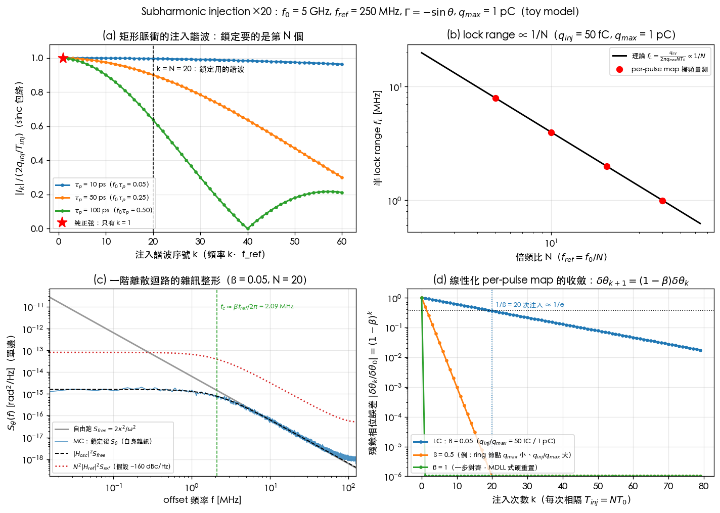
How to read the figure: (a) the horizontal axis of the three sinc envelopes is the harmonic index $k$; the black dashed line $k=N=20$ is the one harmonic the lock actually uses: the 10 ps pulse still has 0.996 there, 100 ps (half a $T_0$) only 0.64, 200 ps (a full $T_0$) zero; the red star is a pure sinusoid — only $k=1$, nothing at $k=20$. (b) The four map-sweep points sit on the $1/N$ line. (c) Grey is the free-running $2\kappa^2/\omega^2$, blue the MC PSD after locking, black dashed $\vert H_{osc}\vert^2S_{free}$: low frequencies are pressed into a $-151$ dBc/Hz plateau, the turnover is at $2.09$ MHz, high frequencies return to free-running; the red dotted line is $N^2\vert H_{ref}\vert^2S_{ref}$ for the assumed $-160$ dBc/Hz reference — 17 dB above the oscillator plateau in-band. (d) $(1-\beta)^k$: $\beta=0.05$ needs 20 pulses to reach $1/e$, $\beta=0.5$ only 1.4, $\beta=1$ one step.

Parameter	Value	Unit	Note
$f_0$, $T_0$	5 GHz, 200 ps	Hz, s	canonical LC
$q_{max}$	1 pC	C	canonical
$\Gamma$	$-\sin\theta$	—	ideal-LC ISF, $\vert\tilde\Gamma_1\vert=1/q_{max}$
$N$, $f_{ref}$, $T_{inj}$	20, 250 MHz, 4 ns	—, Hz, s	multiplication ratio
$q_{inj}$, $\tau_p$	50 fC, 10 ps	C, s	charge and width of each pulse
$\kappa^2$	0.125	rad²/s	canonical (diffusion_dictionary)
$\mathcal{L}_{ref}$	$-160$	dBc/Hz	assumed white reference floor (bookkeeping demo only)
MC length	$2^{20}$ pulses, Welch $2^{14}$	—	about 4.2 ms

Full script: simulations/fig_subharmonic_injection.py (PYTHONPATH=. python3 simulations/fig_subharmonic_injection.py, about 2 s). Pedagogical toy model: phase-only, weak injection, no transistors.

---

5. Design takeaways

5.1 Pulse width vs harmonic content

Fixed area $q_{inj}$: $\vert I_N\vert=\dfrac{2q_{inj}}{T_{inj}}\big\vert\mathrm{sinc}(f_0\tau_p)\big\vert$.

$\tau_p$	$f_0\tau_p$	$\mathrm{sinc}$	$\vert I_{20}\vert$ ($q_{inj}=50$ fC)
10 ps	0.05	0.996	24.90 μA
50 ps	0.25	0.900	22.51 μA
100 ps ($T_0/2$)	0.5	0.637	15.92 μA
200 ps ($T_0$)	1	0	0

The null at $\tau_p=T_0$ has a physical meaning: the pulse spans a whole oscillation period, the positive and negative half-cycles of the ISF cancel, and the locking force vanishes — not "a wider pulse is slightly less efficient", a cliff. Design rule: $\tau_p\ll T_0$ (compared with the output period; larger $N$ means shorter $T_0$ and harder pulses — one of the hard limits of pushing ILCMs to high frequency). The fixed height $I_p$ view (a current-limited driver): $q_{inj}=I_p\tau_p$, $\vert I_N\vert=\frac{2I_p}{\pi N}\sin(\pi f_0\tau_p)$, maximal at $\tau_p=T_0/2$ with $2I_p/(\pi N)$ ($I_p=5$ mA, $N=20$: 159 μA) — the kick efficiency is then 0.64, but the total charge is 10× larger. Both views say: make the pulse a small fraction of $T_0$, but there is no need to push it to the limit — 10 ps already captures 99.6%.

The ring caveat (lab_40 (b)): the single sinc above holds only for "an ISF with just a fundamental". In general the kick is the box average of the ISF over the pulse window, and the $m$-th ISF harmonic is weighted by $\mathrm{sinc}(mf_0\tau_p)$. A ring-type ISF concentrates its energy in triangular pulses about $1/f'$ rad wide ($N_{st}=17$ toy: $0.246$ rad = $0.246/(2\pi)\times200$ ps $\approx7.8$ ps), so the pulse must also be narrower than that width: at the same 10 ps, the LC loses 0.4% while the ring toy's lock range drops to 0.68× (lab_40's unaveraged ODE agrees with the box-average prediction). A ring ILCM needs much narrower pulses than an LC — the flip side of the same node property as "rings win on $q_{max}$".

5.2 Ring vs LC

Section 3's conclusion: $\beta=(q_{inj}/q_{max})\,\vert\Gamma'(\theta_{ss})\vert$. The triangular ISF ties $-\sin$ on slope; the ring's advantage is all in $q_{max}$ ($\times100$). Practical meaning: a ring ILCM can run $\beta\sim0.5$–$1$ (nearly hard realignment every pulse, in-band almost purely reference), an LC only $\beta\sim10^{-2}$ (to stay in weak injection, and because a large $q_{inj}$ kicks the amplitude). An LC ILCM relies on the oscillator being clean (small $\kappa^2$); a ring ILCM relies on frequent, forceful realignment. Section 5.4 quantifies this.

5.3 Choosing $N$ (fixed $f_0$)

Write Section 4's two terms together (time-averaged; the full form for small $\beta$):

$$\sigma_{out}^2(N,\beta)=\underbrace{\kappa^2NT_0\cdot\frac{1-\beta+\beta^2/2}{\beta(2-\beta)}}_{\text{own: random walk between pulses}\ \propto N} +\underbrace{N^2\sigma_\psi^2\cdot\frac{\beta}{2-\beta}}_{\text{reference}\times N^2}$$

• Own term $\propto N$ ($\sigma\propto\sqrt N$): the further apart the pulses, the further the random walk wanders.
• Reference term: $\times N^2$ in the phase domain; but in seconds, $N\sigma_\psi/(2\pi f_0)=\sigma_\psi/(2\pi f_{ref})=\sigma_{t,ref}$ — the reference's time jitter is passed 1:1 to the output, independent of $N$ (rule 1 restated: $\times N$ in phase = the same seconds).
• So for fixed $f_0$ and fixed reference time jitter there is no interior optimum in $N$: smaller $N$ is always better. With $\beta$ re-optimized for each $N$ the script gives, for $N=5,10,20,40,80$, $\sigma_{t,min}=5.99,7.12,8.46,10.07,11.97$ fs, log-log slope $+0.250$ — $\sigma_{t,min}\propto N^{1/4}$ (small-$\beta$ closed form: $\sigma_{min}^2\approx\sigma_w N\sigma_\psi$, $\sigma_w\propto\sqrt N$, $N\sigma_\psi$ fixed ⟹ $\propto N^{1/2}$, then square-root). Doubling $N$ costs only 19% more jitter — the noise penalty of $N$ is mild.
• What really limits $N$ is elsewhere: (i) the lock range $\propto1/N$ (398 ppm at $N=20$) is far below PVT drift ⟹ an FLL is mandatory; (ii) the pulse must be $\ll T_0$; (iii) a clean, high-$f_{ref}$ reference costs money (if the reference is itself multiplied up from a crystal, $S_{ref}\propto f_{ref}^2$ and $N^2S_{ref}$ is independent of $N$ — same conclusion). If an "optimum $N$" exists it is a system-level cost/power optimum, not an extremum of this noise equation.

5.4 The $\beta$ trade-off: noise optimum vs lock range vs spur

Extremize over $\beta$ (small $\beta$: $\sigma_w^2/(2\beta)+N^2\sigma_\psi^2\beta/2$):

$$\beta_{opt}\approx\sqrt{\frac{\sigma_w^2}{N^2\sigma_\psi^2}}=\frac{\sigma_w}{N\sigma_\psi},\qquad \sigma_{out,min}^2\approx\sigma_wN\sigma_\psi$$

— isomorphic to the "optimum loop bandwidth" of pll_noise_budget: VCO noise wants a wide loop, reference noise a narrow one.

Example 5 ($\beta_{opt}$, assumed $-160$ dBc/Hz reference): LC: $\sigma_w=22.4$ μrad, $N\sigma_\psi=20\times158$ μrad ⟹ $\beta_{opt}=0.0071$ (numerical minimization $0.0070$), $\sigma_{out,min}=8.46$ fs (16.3 fs at $\beta=0.05$); corresponding $q_{inj,opt}=7.07$ fC, $\Delta f_L=280$ kHz — a lock range too small to acquire frequency with; this is "the noise-optimal $\beta$ forces you to add an FLL". Ring ($\mathcal{L}(1\text{ MHz})=-100$ dBc/Hz ⟹ $\kappa^2=S_\phi\omega^2/2=3948$ rad²/s, $\sigma_w=3.97$ mrad = 126 fs per $T_{inj}$): $\beta_{opt}=0.695$, $\sigma_{out,min}=123$ fs; 395 fs at $\beta=0.05$, 135 fs at $\beta=1$ — the ring wants a large $\beta$, and its small $q_{max}$ can afford it.

On the spur side (Section 4.4): at fixed detuning the spur is independent of $\beta$; a larger $\beta$ does not worsen it, and a larger $\beta$ = larger lock range = an easier job for the FLL to squeeze $\Delta f_0$. What really grows with $\beta$ is the pulse's direct coupling / AM disturbance (more visible as $q_{inj}$ grows) — outside the first-order phase-only model, honestly left open.

5.5 ILCM vs classic PLL vs sub-sampling PLL

	ILCM (this page)	Classic charge-pump PLL	Sub-sampling PLL (sampling_pll)
Loop	first-order, discrete (one kick per $T_{ref}$)	type-II second-order, continuous approximation	type-II (+ auxiliary FLL)
In-band reference	$N^2S_{ref}$ (rule 1)	$N^2S_{ref}$	$N^2S_{ref}$ (the same)
Divider / CP noise	no divider, no CP; the pulse generator's timing noise enters 1:1 in seconds	$N^2S_{div}+N^2S_{cp}/K_{cp}^2$	divider term gone, CP no longer $\times N^2$
VCO suppression bandwidth	$f_c\approx\beta f_{ref}/2\pi$; with $\beta\to1$ a large fraction of $f_{ref}$	stability-limited to a small fraction of $f_{ref}$ (standard textbook rule of thumb, see pll_noise_budget)	as PLL, but high $K_{PD}$
Frequency acquisition	narrow: $\Delta f_L\propto1/N$ (398 ppm example) ⟹ needs an FLL	wide (the PFD detects frequency)	needs an FLL, harmonic-lock risk
Reference spur	detuning sawtooth $20\log_{10}(\Delta f_0/f_{ref})$, pulse coupling	CP mismatch / leakage	sampler kickback, BW
Lock phase	unique ($\Omega$ has period $2\pi$)	unique	degenerate over $N$ VCO zero crossings (harmonic lock)
Best suited	clean reference + narrow pulses available; ring VCOs with large $\beta$	general purpose	low in-band, FLL budget available

5.6 Connection to SerDes

Forwarded-clock architectures often take a low-rate forwarded clock (e.g. $f_0/4$ or $f_0/8$) and multiply it back to full rate at the receiver with an ILO / ILCM: this page's $f_c$ is the jitter-tracking bandwidth — reference (forwarded-clock) jitter below $f_c$ is copied onto the local clock (good for common jitter: transmitter and receiver correlate and cancel), above $f_c$ the local oscillator is on its own ($\kappa^2$, i.e. the old $\Gamma_{rms}/q_{max}$ homework). The trade-off has the same structure as item 5 of injection_locking_noise and serdes_clocking_connection, only with $N\gt1$ and discrete updates.

---

6. Worked numbers: one Python block computes everything (canonical values)

import numpy as np
f0, qmax, kappa2 = 5e9, 1e-12, 0.125          # Hz, C, rad^2/s (canonical)
N, qinj, tau_p = 20, 50e-15, 10e-12           # multiplication ratio, injected charge [C], pulse width [s]
fref = f0/N; Tinj = 1/fref                    # 250 MHz, 4 ns
I_N = 2*qinj/Tinj*abs(np.sinc(N*fref*tau_p))  # N-th injection harmonic amplitude [A] (sinc argument = f0*tau_p)
wL  = 0.5*I_N*(1/qmax)                        # route 1: (1/2)|I_N||Gt_1| [rad/s]
beta = qinj/qmax*abs(np.sinc(f0*tau_p))       # realignment factor (lock-range centre, incl. pulse width)
fc  = beta*fref/(2*np.pi*(1-beta))            # corner [Hz]
sw2 = kappa2*Tinj                             # phase variance accumulated per T_inj [rad^2]
var_avg = sw2*(1-beta+beta**2/2)/(beta*(2-beta))
S_ref = 2*10**(-160/10); sig_psi2 = S_ref*fref/2   # assumed -160 dBc/Hz white reference
var_ref = beta*N**2*sig_psi2/(2-beta)
b_opt = np.sqrt(sw2/(N**2*sig_psi2))
print(I_N*1e6)                                # -> 24.90 μA
print(wL, wL/2/np.pi/1e6)                     # -> 1.245e7 rad/s, 1.981 MHz
print(qinj/(qmax*Tinj)/2/np.pi/1e6)           # -> 1.989 MHz (impulse route, sinc=0.996 apart)
print(beta, -1/np.log(1-beta))                # -> 0.0498, 19.58 injections (to 1/e)
print(fc/1e6)                                 # -> 2.085 MHz
print(np.sqrt(var_avg)*1e6, np.sqrt(var_avg)/(2*np.pi*f0)*1e15)  # -> 69.99 μrad, 2.228 fs
print(10*np.log10(2*kappa2*Tinj**2/beta**2/2))                    # -> -150.9 dBc/Hz own-noise plateau
print(np.sqrt(var_ref)/(2*np.pi*f0)*1e15, 10*np.log10(N**2*S_ref/2))  # -> 16.08 fs, -134.0 dBc/Hz reference in-band
print(b_opt, b_opt*qmax*1e15)                 # -> 0.00707, 7.07 fC
print(20*np.log10(100e3/fref))                # -> -67.96 dBc (f_ref spur for a 100 kHz detuning)

($\beta=0.0498$ includes the sinc of the 10 ps pulse; the table in Section 4 uses the delta train's $\beta=0.05$, 0.4% apart.)

---

Applicability and failure conditions

Condition	When it holds	When it fails
Weak injection $q_{inj}\ll q_{max}$ ($\beta\ll1$)	linear kick, $\Delta\phi=\tilde\Gamma q_{inj}$, first-order average of [P4] Eq.(29) valid	large kicks: use the $2\sin^{-1}$ of [P3] footnote 9, asymmetric lock range; hard realignment at $\beta\to1$ (ring / MDLL) is still described by the map, but the linear $\Omega(\theta)$ loses accuracy
Injection carries its own $N$-th harmonic (pulses)	$\omega_L=\tfrac12\vert I_N\vert\vert\tilde\Gamma_1\vert$	pure sinusoid: $\vert I_N\vert=0$, no first-order lock; locking via internal mixing is outside the framework, as [P4] footnote 10 states
$\theta$ slowly varying within one $T_{inj}$	time-synchronous average / discrete bookkeeping of the map valid	large detuning (beyond $\Delta\omega_L$): cycle slips, pulling comb (injection_locking_noise Part B)
Phase-only	everything on this page	the zero-detuning LC lock point is the waveform peak, where pulses kick the amplitude ([P4] APF); large $q_{inj}$ needs the AM correction
White frequency noise ($\kappa^2$)	$\sigma_w^2=\kappa^2T_{inj}$, closed-form variances	flicker FM: intra-interval variance no longer $\propto t$, the closed forms need a different kernel; minor when in-band is reference-limited
$f\ll f_{ref}/2$	discrete $\vert H\vert^2$ = continuous first-order PLL	near $f_{ref}/2$: sampling effects, $\vert1-z^{-1}\vert^2\to4$; this page compares only for $f\lt f_{ref}/8$ (MC/theory 1.03)
First-order sawtooth spur	$20\log_{10}(\Delta f_0/f_{ref})$	pulse feedthrough, AM, pulse width, nonlinear kicks not included; measured spurs are often dominated by these
Triangular ring ISF toy	slope $=1$, dead zone	real ring ISF flanks are not strictly triangular, dead zones not strictly zero; the $q_{max}$ order-of-magnitude conclusion ($\times100$) stands

Key takeaways

• [P4] writes out only the superharmonic Eq.(30); the subharmonic (multiplier) closed form follows from Eq.(29): selection rule $k=mN$, $\Omega(\theta)=I_0\tilde\Gamma_{dc}+\tfrac12\sum_m\vert\tilde\Gamma_m\vert\vert I_{mN}\vert\cos(m\theta+\cdots)$, fundamental-dominated $\omega_L=\tfrac12\vert I_N\vert\vert\tilde\Gamma_1\vert$. Division rides on ISF harmonics, multiplication on injection harmonics; a pure sinusoid at $f_0/N$ cannot lock to first order.
• The arithmetic of [P3] footnote 7: one kick every $N$ periods, $\Delta\omega_L=q_{inj}\vert\tilde\Gamma\vert_{max}/(NT_0)\propto1/N$; a delta train's harmonics have equal weight ⟹ exactly equal to the Fourier route ($\Omega=q_{inj}\tilde\Gamma(\theta)/T_{inj}$). A finite pulse width multiplies by $\mathrm{sinc}(f_0\tau_p)$ — compared with $T_0$, not $T_{inj}$.
• $\beta=-q_{inj}\tilde\Gamma'(\theta_{ss})$: the fraction one pulse pulls back; stable for $0\lt\beta\lt2$, settles in $\approx1/\beta$ injections; $\beta/T_{inj}=\omega_c=-\Omega'(\theta_{ss})$ (the pull-in frequency of [P3] Eq.(40)), $=\Delta\omega_L$ for the LC at centre. The ring does not win on slope (the triangular toy ties at slope $=1$); it wins on a 100× smaller $q_{max}$.
• Noise: $H_{ref}=\beta/(1-(1-\beta)z^{-1})$, $H_{osc}=(1-z^{-1})/(1-(1-\beta)z^{-1})$; in-band reference $\times N^2$ ($+26$ dB at $N=20$), own-noise plateau $2\kappa^2T_{inj}^2/\beta^2$, corner $\approx\beta f_{ref}/2\pi$, out-of-band back to free-running ($\times1/(1-\beta)^2$). Closed-form output variance $\kappa^2NT_0(1-\beta+\beta^2/2)/(\beta(2-\beta))$ (MC ratio 0.999; canonical 2.22 fs).
• Spur: detuning sawtooth $20\log_{10}(\Delta f_0/f_{ref})$ (100 kHz → $-68$ dBc), first order, independent of $\beta$.
• Design: pulse width $\ll T_0$; $\beta_{opt}=\sigma_w/(N\sigma_\psi)$ is often so small that the lock range cannot cover PVT ⟹ add an FLL; the noise penalty of $N$ is only $N^{1/4}$ — what limits $N$ is the $1/N$ lock range, pulse speed and reference cost.

Further reading

• The impulse-train thought experiment and Eq.(19)–(23) step by step: paper_003 ([P3] Sec. IV, p.2112; footnotes 7, 9)
• Origin of the M:N averaging equation and the superharmonic closed form: paper_004 ([P4] Eq.(28)–(30), p.2129; footnote 10)
• The other half of the duality — division rides on the ISF's $N$-th harmonic, half-wave symmetry cannot divide by 2: injection_locked_division
• Locked oscillator = first-order PLL, corner $=-\Omega'(\theta_{ss})$, pulling comb: injection_locking_noise
• The $+20\log_{10}N$ of ×$N$ and the PLL's $N^2S_{ref}$: clock_chain_budget rules 1, 3
• The other way to kick the divider out of the loop: sampling_pll; the second-order version of the optimum loop bandwidth: pll_noise_budget
• ÷2 ILFD for quadrature and the first appearance of the ILFD / multiplier duality: quadrature_and_coupled_oscillators
• The five costumes of $\kappa^2$ (source of this page's $\sigma_w^2=\kappa^2T_{inj}$): diffusion_dictionary
• Independent simulation: lab_40_subharmonic_injection

External literature (not in the 5 downloaded PDFs; authorship, volume and pages verified separately)

• [E-Ye02] S. Ye, L. Jansson, and I. Galton, "A Multiple-Crystal Interface PLL With VCO Realignment to Reduce Phase Noise," IEEE J. Solid-State Circuits, vol. 37, no. 12, pp. 1795–1803, Dec. 2002. (The classic on VCO realignment: periodically injection-locking a PLL's VCO to a buffered reference, effectively widening the loop bandwidth; one of the standard sources for this page's $\beta$ and first-order discrete noise shaping.)
• [E-Lee09] J. Lee and H. Wang, "Study of Subharmonically Injection-Locked PLLs," IEEE J. Solid-State Circuits, vol. 44, no. 5, pp. 1539–1553, May 2009. (A complete analysis of subharmonically injection-locked PLLs: noise shaping, lock range, PVT tolerance and pseudo-locking — the practical background for Section 5.4's "the noise-optimal $\beta$ forces you to add an FLL".)
• [E-Gao09] X. Gao, E. A. M. Klumperink, M. Bohsali, and B. Nauta, "A Low Noise Sub-Sampling PLL in Which Divider Noise Is Eliminated and PD/CP Noise Is Not Multiplied by N²," IEEE J. Solid-State Circuits, vol. 44, no. 12, pp. 3253–3263, Dec. 2009. (The sub-sampling column of the table in Section 5.5; already cited on the site's sampling_pll.)