β: This English translation is in beta — the Traditional-Chinese original is the authoritative version.

Injection-Locked Frequency Division (ILFD): M:N Sub-/Super-Harmonic Locking and Design

Prerequisites: paper_004 (the original, fully worked derivation of [P4] Eq.(28)-(30), p.2129 — this page is a teaching summary and extension of it), fourier_series_of_isf (the ISF's Fourier coefficients and symmetry table, the skeleton for this page's payoff) | Next: subharmonic_injection (the dual story: sub-harmonic injection / multipliers), injection_locking_noise (noise shaping of a locked oscillator, whose framework this page's last section borrows)

What this page answers:

1. Why use an injection-locked frequency divider (ILFD) instead of a digital divider?
2. Where does the ÷$N$ lock-range formula come from, and which ISF harmonic sets it?
3. Why can a differential, half-wave-symmetric oscillator not divide by 2 in the first place? How do you design around it?
4. How should you account for the phase noise of a divided output — a clean $-20\log_{10}N$, or something else?

Physical intuition (the punchline first): an ILFD is not a "division circuit" — it is an oscillator that already runs at $f_0=f_{inj}/N$, and the injection current gives its phase a small tug once per oscillation cycle, locking it to exactly $1/N$ of the input. How hard that tug pulls depends on how much content the oscillator's own ISF has at its $N$-th harmonic — this is the first place on this site where [P1] Eq.(12)'s Fourier expansion is genuinely used as a design knob: the ISF's harmonics don't just decide how noise folds back onto the carrier — they also decide whether the divider locks at all.

---

Why injection-locked division instead of a static divider

High-speed local-oscillator chains (e.g., the first divider stage in an mm-wave PLL) typically choose between:

1. A static digital divider (CML latches, TSPC/D-flip-flop chains; the ÷2 section of quadrature_and_coupled_oscillators already covers this route): every stage must toggle correctly at the full input rate, so dynamic power scales up with input frequency and the process needs comfortable switching margin at that frequency — the closer the input frequency sits to the process limit, the steeper the power and reliability cost.
2. An ILFD (this page's subject): fundamentally an oscillator that runs at its own $f_0$ (not $f_{inj}$); it only needs an injection current, much smaller than its own oscillation amplitude, to "hold" its phase — it never has to toggle logic at the full $f_{inj}$ rate, only oscillate at its own native $f_0$ and let the injection path (often just a capacitor or a small transistor window, not a full toggling stage) tolerate $f_{inj}$. This typically lets an ILFD run cheaper on power and reach higher frequencies as the input approaches the process limit — which is why it is popular as the front divider stage in mm-wave PLLs.

Honesty note: the above is standard analog/RF design lore (external knowledge, not a quantitative result from any of the 5 site PDFs); [P4] never gives a power comparison between an ILFD and a static divider. This section is qualitative reasoning only. A quantitative comparison would need to cite a specific process/topology paper (TODO: unverified). What follows is the rigorous math [P4] does give: whether an ILFD locks, and how wide.

---

The M:N generalized averaging equation: how the ISF's $N$-th harmonic gets "grabbed"

[P3]'s generalized Adler equation only handles an injection frequency $\omega_{inj}\approx\omega_0$ (fundamental locking). [P4] Sec. IV (Eq.(28)-(30), p.2129, verified against the original PDF on this site; see paper_004 for the complete step-by-step version) generalizes this to an arbitrary rational frequency ratio: under lock, $M\omega_{inj}=N\omega_{osc}$ ($M,N$ coprime positive integers). ILFD is the $M=1$ special case (output $=\omega_{inj}/N$, i.e., division); $N=1$ is the injection-locked frequency multiplier (multiplication). The derivation below is compressed to three steps; see [paper_004] for the full version.

Step 1 (re-define the relative phase, Eq.(28)):

$$\varphi(t)\equiv\frac{M}{N}\,\omega_{inj}t+\theta(t)$$

$\varphi$ is the oscillator's total phase [rad], and $\theta$ is the slowly varying phase relative to the injection clock [rad]. A ÷2 ILFD takes $M=1,N=2$: inject at $\omega_{inj}\approx2\omega_0$, and the oscillator runs at $\omega_{inj}/2$.

Step 2 (time-synchronous average over an $NT_{inj}$ window, Eq.(29)):

$$\frac{d\theta}{dt}=\omega_0-\frac{M}{N}\omega_{inj}+\frac{1}{NT_{inj}}\int_{NT_{inj}}\tilde\Gamma\!\left(\frac{M}{N}\omega_{inj}t+\theta\right)i_{inj}(t)\,dt$$

The window is $NT_{inj}$ (not $T_{inj}$) because: within the window the injection waveform completes $N$ full cycles, and the ISF's argument advances by $(M/N)\,\omega_{inj}\cdot NT_{inj}=2\pi M$, i.e., $M$ full cycles — both are integer numbers of cycles, which is exactly what makes the averaging clean.

Step 3 (term-by-term averaging — only the resonant harmonic survives, giving Eq.(30)): take $M=1$ and a sinusoidal injection $i_{inj}=I_{inj}\cos(\omega_{inj}t)$, and expand $\tilde\Gamma$ as a phasor Fourier series (matching [P1] Eq.(12): $\vert\tilde\Gamma_n\vert=c_n/q_{max}$, units rad/C). Multiplying term by term and applying the product-to-sum identity, every term except the $n=N$ difference-frequency term (whose frequency is exactly 0) completes an integer number of cycles over the $NT_{inj}$ window and averages exactly to zero — this is an identity, not "approximately small" (lab_37 below verifies it numerically to $10^{-15}$). The one surviving term:

$$\Omega(\theta)=\frac{1}{2}\,I_{inj}\,\vert\tilde\Gamma_N\vert\cos\!\big(N\theta+\angle\tilde\Gamma_N\big)$$

Reading it: only the oscillator's ISF $N$-th harmonic $\vert\tilde\Gamma_N\vert$ responds to injection at the $N$-th superharmonic — not the fundamental $\vert\tilde\Gamma_1\vert$, and not any other harmonic. ÷2 uses $\vert\tilde\Gamma_2\vert$ (i.e., $c_2$); ÷3 uses $\vert\tilde\Gamma_3\vert$ (i.e., $c_3$).

---

Lock range: $\omega_L=\tfrac12 I_{inj}\vert\tilde\Gamma_N\vert$ — carried by the ISF's $N$-th harmonic

Locking $\Leftrightarrow d\theta/dt=0$ has a stable solution $\Leftrightarrow\vert\Delta\omega\vert\le\max_\theta\Omega(\theta)$ ($\Delta\omega\equiv\omega_{inj}/N-\omega_0$, on the output frequency axis). [P4] p.2130, verbatim: "which can be calculated from (30) to be $\omega_L=I_{inj}\vert\tilde\Gamma_N\vert/2$":

$$\omega_L=\frac{1}{2}\,I_{inj}\,\vert\tilde\Gamma_N\vert=\frac{I_{inj}\,c_N}{2\,q_{max}}$$

Three pieces of physics you can read off immediately ([P4] p.2129-2130, verified):

1. The division ratio $N$ does not appear directly in the formula — it only selects which harmonic $c_N$ is used; the ÷2 and ÷3 lock ranges fall on one and the same $f_L\propto c_N$ line (see lab_37 panel (b) below).
2. $\omega_L$ is reckoned on the output frequency axis; converted to the injection-frequency axis, the lockable $\omega_{inj}$ window is $2N\omega_L$ wide.
3. $\Omega(\theta)$ has period $2\pi/N$ ⟹ there are $N$ stable locked phases spaced $2\pi/N$ apart that are mutually indistinguishable — a ÷$N$ output has $N$ possible phase startpoints (output phase ambiguity), which must be handled separately for multi-phase clocking.

Example (÷2 ILFD: 10 GHz in, 5 GHz out, canonical values, replayed from [paper_004]): $f_0=5$ GHz, $q_{max}=1$ pC, a sinusoidal injection of $I_{inj}=0.5$ mA at $f_{inj}\approx10$ GHz, and ISF second harmonic $c_2=0.5$.

1. $\vert\tilde\Gamma_2\vert=c_2/q_{max}=0.5/10^{-12}=5\times10^{11}$ rad/C.
2. $\omega_L=\tfrac12 I_{inj}\vert\tilde\Gamma_2\vert=\tfrac12(5\times10^{-4}\,\text{A})(5\times10^{11}\,\text{rad/C})=1.25\times10^{8}$ rad/s.
3. $f_L=\omega_L/2\pi=19.9$ MHz (only $0.40\%$ of $f_0$); the lockable window on the injection-frequency axis is $2Nf_L=79.6$ MHz.
4. Dimension check: A $\times$ rad/C $=$ rad/s ✓. Weak-injection check: $I_{max}:=\omega_0 q_{max}=31.4$ mA ([P4] footnote 11, p.2130), $I_{inj}/I_{max}=1.6\%$ ⟹ the first-order linear model applies.

One-line Python: 0.5*0.5e-3*0.5/1e-12 → $1.25\times10^{8}$.

Quick check (work it out yourself, then check)

Work it out yourself first: swap the same oscillator to ÷3 (N=3, c_3=0.2, I_inj=0.5 mA, q_max=1 pC). Using ω_L=I_inj·c_N/(2·q_max), what is the half lock range f_L (MHz, round to 2 decimals)?

MHz

Graded correct within ±5% relative error; scientific notation is accepted.

---

A half-wave-symmetric ISF cannot divide by 2 (the payoff)

Look back at the symmetry table in Step 7 of fourier_series_of_isf: half-wave symmetry $\Gamma(x+\pi)=-\Gamma(x)$ ⟹ the even harmonics $c_2=c_4=\dots=0$. Substitute into $\omega_L=I_{inj}c_2/(2q_{max})$: the ÷2 lock range is identically zero — to first order, no matter how large you make $I_{inj}$, an injection at $2f_0$ simply will not lock.

This is the same symmetry table telling two different stories: on the phase-noise side (white_noise_to_phase_noise) it's good news — noise near $2\omega_0$ does not fold back onto the carrier; on the ILFD side it's bad news — symmetry is a double-edged sword. An ideal differential LC VCO's differential output nodes are exactly this case ($c_2\approx0$). The design way out is to change the injection node — the ISF is "one curve per injection node" (as in [P1]); differential outputs are symmetric, but certain internal nodes are naturally asymmetric — the next section covers this in detail.

---

Numerical verification: lab_37 (unaveraged-ODE sweeps + harmonic maps)

lab_37 integrates the unaveraged instantaneous equation directly (verifying the already-averaged Eq.(30) with Eq.(30) itself would be circular):

$$\frac{d\theta}{dt}=\Big(\omega_0-\frac{\omega_{inj}}{N}\Big)+\tilde\Gamma\!\Big(\frac{\omega_{inj}}{N}t+\theta\Big)\,I_{inj}\cos(\omega_{inj}t)$$

The ISF is a 3-harmonic toy (pedagogical toy, not transistor-level): $\tilde\Gamma(x)=-\big(c_1\sin x+c_2\sin2x+c_3\sin3x\big)/q_{max}$.

Parameter	Value	Units
$f_0$	5	GHz
$q_{max}$	1	pC
$I_{inj}$	0.5	mA
$(c_1,c_2,c_3)$	$(1.0,\,0.5,\,0.2)$	—
ODE step / total time	1 ps / 600 ns	—
Theory $f_L$ ($N=2$, $c_2=0.5$)	19.89	MHz
Theory $f_L$ ($N=3$, $c_3=0.2$)	7.96	MHz

PYTHONPATH=. python simulations/lab_37_ilfd_lock.py
# -> 1.13e-15 / 3.19e-15 (max relative error of the numerical average of Eq.(29) vs the closed form Eq.(30), N=2 / N=3: identity-level)
# -> 1.033 (2f0 sweep: measured omega_L / theory 1.25e8 rad/s; the 61-point grid resolves ~3%)
# -> 1.000 (3f0 sweep: measured omega_L / theory 5e7 rad/s)
# -> 0/61 (locked points of the half-wave-symmetric c2=0 ISF on the same +/-2 omega_L grid: never locks, no /2)
# -> 1.004 / 1.019 (mean measured/theory ratio of the lock range swept vs c2 (N=2) and vs c3 (N=3): linearity holds)
# -> 1.000 (out-of-lock mean drift rate / (omega_b/N), [P4] Eq.(34))
# -> 3.1330 (gap between converged phases from two initial conditions at N=2, theory 2pi/2=3.1416: the 2pi/N degeneracy)

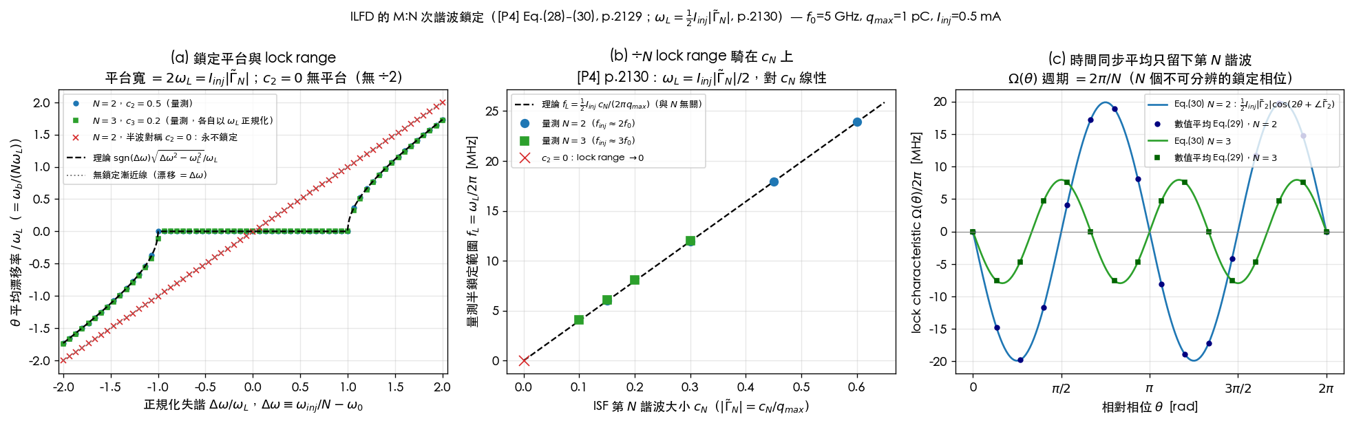
How to read it (full script: simulations/lab_37_ilfd_lock.py, runtime ≈ 19 s; full panel-by-panel walkthrough is in paper_004):

• (a): locking = the zero-drift plateau, whose half-width is exactly $\omega_L$; the red $c_2=0$ (half-wave-symmetric) curve is a straight line through the origin (drift = detuning) — it never locks at any detuning, 0/61 grid points locked.
• (b): the $N=2$ and $N=3$ measured points fall on one and the same theory line $f_L=I_{inj}c_N/(4\pi q_{max})$ ($N$ only selects the harmonic; it does not enter the formula).
• (c): the averaging integral of Eq.(29) evaluated numerically for each $\theta$, overlapping the closed form Eq.(30); period $\pi$ for $N=2$ and $2\pi/3$ for $N=3$ — the $2\pi/N$ degeneracy visible to the naked eye.

---

Design notes: how to create $c_2$ so ÷2 can lock

"Half-wave symmetry can't divide by 2" is not a death sentence — it's a hint that the injection node needs to change. Two routes:

1. Break the half-wave symmetry itself: half-wave symmetry $\Gamma(x+\pi)=-\Gamma(x)$ requires that the "rising half-cycle" and "falling half-cycle" of the waveform be mirror-image, opposite-sign copies of each other — a differential, push-pull node naturally satisfies this (two complementary switching events, opposite polarity, half a period apart). A single-ended node typically does not: a period often contains only one dominant sensitivity event (e.g., the CMOS ring-inverter stage derived in real_oscillator_topologies section (c): the ISF concentrates in a single transition window, not two mirror-image windows), or the rise and fall edges' slope and timing are simply not symmetric to begin with (the Colpitts case in the same page's section (b)). Such topologies do not automatically satisfy $\Gamma(x+\pi)=-\Gamma(x)$, and $c_2$ is naturally nonzero — this is the mechanism behind "asymmetric/single-ended topologies are easier to divide by 2."
2. Move to a node that is naturally asymmetric — tail injection at $2f_0$: a differential LC VCO's differential output is symmetric with $c_2\approx0$, but section (a) of real_oscillator_topologies already works out that the tail node's effective ISF is rich in $c_2$: because the switching pair "flips" the tail current twice per cycle, the tail node voltage naturally swings at $2\omega_0$, and $\Gamma_{tail}(\theta)=\tfrac{c_0}{2}+c_{1,res}\cos\theta+c_2\cos2\theta$ takes $c_2=0.55$ in that page's illustrative model — much larger $c_2$ content than the tank's $c_1=1,c_2=0$. [P4]'s own ÷2 experiments inject $2f_0$ precisely into the tail of a differential LC (Fig. 11(a)(b) caption and Fig. 12(d), p.2130-2131, verified) — matching, independently, what real_oscillator_topologies already establishes as "the tail is where $c_2$ lives": that page discusses the same $c_2$ folding back tail noise; this page uses the very same $c_2$ for active injection locking — two sides of one coin.

Design-knob summary:

1. To make ÷2 lock, find a node not protected by differential symmetry to inject into (the tail, or an auxiliary single-ended node).
2. If that node is also the source of $c_2$ fold-back noise (as the tail is), you're "borrowing the same weakness" — injection locking uses it to help divide, but during normal operation it is also folding $2\omega_0$ noise back; the frequency a tail filter (see real_oscillator_topologies) normally wants to filter out is exactly the frequency you want to inject for locking — these two need to be designed with time- or frequency-domain separation, not left to fight each other.
3. Single-ended topologies (ring inverters, Colpitts) already have nonzero $c_2$, making ÷2 ILFD relatively easy — but note that their $\Gamma_{rms}$ and $c_0$ characteristics (sections (b)(c) of real_oscillator_topologies) come along for the ride too; you don't get to cherry-pick only the $c_2$ term.

---

Duality: division spends ISF harmonics, multiplication needs injection harmonics

[P4] Eq.(28)'s general $M:N$ form actually describes a pair of mirror-image relationships; this site has only fully verified and derived the $M=1$ (division) half. Swapping the roles of $M$ and $N$ reveals the duality:

	÷$N$ (ILFD, this page, $M=1$)	×$M$ (injection-locked multiplier, $N=1$)
Lock condition	$M=1\Rightarrow\omega_{osc}=\omega_{inj}/N$	$N=1\Rightarrow\omega_{osc}=M\,\omega_{inj}$
Who must supply the harmonic	The oscillator's ISF supplies the $N$-th harmonic $\vert\tilde\Gamma_N\vert$; the injection itself only needs its fundamental $\cos(\omega_{inj}t)$	The injection waveform must supply its own $M$-th harmonic; the ISF only needs its fundamental $\vert\tilde\Gamma_1\vert$
How it's built	A plain sinusoidal current injection is enough ($N$-th-order content all comes from the ISF's own Fourier expansion)	A pure sinusoid has no $M\ge2$ harmonics, so in practice they must be generated by mixing inside the oscillator — [P4] footnote 10, p.2129 explicitly states this is not captured by the Eq.(28)-(30) framework (partially handled by its reference [25])
Lock-range formula	$\omega_L=\tfrac12 I_{inj}\vert\tilde\Gamma_N\vert$ (this page's Eq.(30), verified)	Depends on the internal mixing gain; no closed form of this kind (beyond what this site has verified)

Duality in one line: a divider outsources the work to the oscillator's own spectral content (ISF harmonics); a multiplier instead needs the injection signal to already have high-order harmonics — and "making a sinusoid grow harmonics" is exactly the problem subharmonic_injection works through (sub-harmonic injection / multipliers, and how they generate the needed $M$-th harmonic drive in practice). Both pages share the same formula skeleton ([P4] Eq.(28)) — the only difference is which side the harmonic content lives on.

---

Noise accounting: the divider's $-20\log_{10}N$ meets the locked oscillator's own noise shaping

clock_chain_budget Rule 2 rigorously derives the phase accounting for an ideal ÷$N$ (edge-picking — the divider only discards edges, it never moves them): $\phi_{out}=\phi_{in}/N\Rightarrow\mathcal{L}_{out}=\mathcal{L}_{in}-20\log_{10}N$. That page's "Relationship to [P4]" callout already points out that the ÷$N$ phase accounting ($\phi/N$) also holds for the ILFD's carrier path — and the reason lies right here, in this page's Eq.(28): with $M=1$, $\varphi(t)=\omega_{inj}t/N+\theta(t)$, and $\theta$ is a bounded, slowly varying quantity within the lock range, so the deterministic carrier-frequency relationship $\omega_{out}=\omega_{inj}/N$ is itself an exact $1/N$ scaling — the same statement as clock_chain_budget Rule 2's $\phi_{out}=\phi_{in}/N$, just with a whole locked oscillator standing in for the logic gate.

But an ILFD is not a pure edge-picking machine — it is a locked oscillator — which is exactly the part clock_chain_budget honestly leaves open: "near the edge of the lock range, an ILFD has its own noise behavior." That other half connects to the framework of injection_locking_noise, which proves, for fundamental locking ($M=N=1$), that a locked oscillator's own noise is high-pass shaped, with corner defined as $\omega_c\equiv-\Omega'(\theta_{ss})$ (the slope of the lock characteristic at the stable point). Applying that same definition to this page's $M:N$ version, $\Omega(\theta)=\tfrac12 I_{inj}\vert\tilde\Gamma_N\vert\cos(N\theta+\angle\tilde\Gamma_N)$:

$$\Omega'(\theta)=-N\,\omega_L\sin\!\big(N\theta+\angle\tilde\Gamma_N\big) \quad\Longrightarrow\quad \omega_c=\big\vert\Omega'(\theta_{ss})\big\vert=N\,\omega_L\sqrt{1-\Big(\frac{\Delta\omega}{\omega_L}\Big)^{2}}=N\sqrt{\omega_L^2-\Delta\omega^2}$$

(using the lock condition $\cos(N\theta_{ss}+\angle\tilde\Gamma_N)=\Delta\omega/\omega_L$. Dimension check: $\omega_L$ is rad/s, $N$ is dimensionless ⟹ $\omega_c$ is rad/s ✓.) This $\omega_c$ is exactly the already-verified pull-in frequency $\omega_p=N\sqrt{\omega_L^2-\Delta\omega^2}$ of [P4] Eq.(32) — not a coincidence, but the same fact: applying injection_locking_noise's general principle "the noise corner is the restoring force of the lock characteristic" to the $M:N$ version of $\Omega(\theta)$ automatically reproduces the paper's own already-verified transient time constant.

The design picture that joins the two halves:

• Offset frequency $\ll\omega_c$ (inside the loop bandwidth): $\theta$ tracks the injection source closely, and the carrier-path accounting $\phi_{out}=\phi_{in}/N$ holds — the output inherits the phase noise of the injection source (the upstream $f_{inj}$ clock), echoing, in magnitude, the $-20\log_{10}N$ intuition of clock_chain_budget Rule 2 (think of "$-20\log_{10}N$" as "the carrier is deterministically divided by $N$," not as "the divider actively suppresses noise").
• Offset frequency $\gg\omega_c$ (outside the loop bandwidth): $\theta$ can no longer keep up, and the ILFD's own free-running phase noise (its own $\Gamma_{rms}/q_{max}$, the familiar [P1] Eq.(21)) dominates the output through the high-pass $S_n/(\omega_c^2+\omega^2)$ — here $-20\log_{10}N$ no longer applies, and the output noise is set by the quality of the ILFD oscillator itself.
• The closer to the edge of the lock range ($\Delta\omega\to\omega_L$), the smaller $\omega_c\to0$ becomes — the high-pass corner retreats to lower frequency and the suppression bandwidth shrinks. This is the same honest reminder as clock_chain_budget Rule 4's "the divider's own noise floor": a real ILFD has its own noise floor too, and the output can never be better than the ILFD's own noise behavior at that offset frequency.

---

Applicability / failure conditions

Condition	When it holds	What happens when it fails
Weak injection $I_{inj}\ll I_{max}=\omega_0 q_{max}$ ([P4] footnote 11, p.2130)	First-order averaging, the $\omega_L$ formula, hold	Strong injection: needs the APF correction (Eq.(27) denominator) and amplitude dynamics; the first-order formula loses accuracy
$\omega_L\ll\omega_0$	The averaging (Eq.(29)) holds	Detuning too large, or the oscillator dynamics too fast within the averaging window: the averaging breaks down
$M=1$ (this page covers only the division direction)	Eq.(30)'s closed form holds	$M\neq1$ (multiplication) needs the $M$-th harmonic of the injection signal, which a sinusoidal injection lacks — [P4] footnote 10 explicitly says this is outside the framework; see the duality table above
"$c_2=0$ cannot divide by 2"	A first-order conclusion	Higher-order mixing may still leave a tiny residual lock range (below lab_37's detection floor)
The high-pass/low-pass part of the noise accounting	Standard injection-locking noise theory (injection_locking_noise)	Not covered by the 5 site PDFs (Kurokawa 1973; [P4] p.2130 points to its reference [29, Ch. 7]); this page applies the general definition of $\omega_c$ to the $M:N$ case, and the resulting value numerically matches [P4]'s already-verified Eq.(32)

What to remember

• An ILFD is a locked oscillator, not a logic divider: it locks its phase to $\omega_{inj}/N$ via injection current, without needing to switch logic at the full $f_{inj}$ rate — the qualitative reason it saves power as a high-frequency front-end stage.
• The math of locking ([P4] Eq.(28)-(30), p.2129, verified): time-synchronous averaging over an $NT_{inj}$ window keeps only the ISF's $N$-th harmonic, giving $\Omega(\theta)=\tfrac12 I_{inj}\vert\tilde\Gamma_N\vert\cos(N\theta+\angle\tilde\Gamma_N)$, with lock range $\omega_L=\tfrac12 I_{inj}\vert\tilde\Gamma_N\vert=I_{inj}c_N/(2q_{max})$ — the division ratio $N$ only picks the harmonic, it does not enter the formula; there are $N$ locked phases spaced $2\pi/N$ apart that are mutually indistinguishable.
• The payoff: half-wave symmetry $\Rightarrow c_2=c_4=\dots=0\Rightarrow$ the ÷2/÷4 lock range is identically zero to first order — a differential output node cannot divide by 2; the way out is to inject into an asymmetric node (the tail, or an auxiliary single-ended node) instead.
• lab_37: the unaveraged ODE directly verifies the averaging identity to $10^{-15}$, measured lock ranges match theory at a ratio of 1.00-1.03, the $c_2=0$ case locks at 0/61 grid points, and the $2\pi/N$ degeneracy is visible to the naked eye.
• Creating $c_2$ by design: break half-wave symmetry (single-ended/asymmetric topologies naturally have nonzero $c_2$) or move the injection node (a differential LC VCO's tail is naturally rich in $c_2$ — the same mechanism as tail-noise fold-back, seen from the other side).
• Duality: division ($M=1$) spends the oscillator's own ISF harmonics; multiplication ($N=1$) needs the injection signal's own harmonics — a sinusoidal injection has none, so internal mixing is required, which is outside this framework (see subharmonic_injection).
• Noise: the carrier-path accounting $\phi_{out}=\phi_{in}/N$ holds for an ILFD (echoing clock_chain_budget Rule 2's $-20\log_{10}N$); but beyond the loop bandwidth $\omega_c=N\sqrt{\omega_L^2-\Delta\omega^2}$ (exactly [P4] Eq.(32)'s pull-in frequency), the output noise is set by the ILFD's own free-running phase noise, high-pass shaped — not a simple $-20\log_{10}N$.

Further reading

• The complete step-by-step derivation and experimental evidence: paper_004 ([P4] Eq.(28)-(30), p.2129; $\omega_L$, p.2130; transient Eq.(31)-(34), p.2130; experiments Fig. 11-12, p.2130-2131)
• The ISF's Fourier expansion and symmetry table (the skeleton of this page's payoff): fourier_series_of_isf
• ÷2's first appearance as a quadrature generator, and its contrast with a static divider: quadrature_and_coupled_oscillators
• ISF harmonics of three real topologies (the source of this page's "how to create $c_2$" numbers): real_oscillator_topologies
• The rigorous origin of the ÷$N$ phase accounting $-20\log_{10}N$: clock_chain_budget Rule 2
• High-pass shaping of a locked oscillator's own noise (the framework this page's last section borrows): injection_locking_noise
• The other half of the duality — sub-harmonic injection / multipliers: subharmonic_injection