β: This English translation is in beta — the Traditional-Chinese original is the authoritative version.

A General Theory of Injection Locking and Pulling in Electrical Oscillators—Part II

Prerequisites (recommended reading order): paper_001 (the ISF $\Gamma$ is the tangential projection) → phase_vs_amplitude_noise (why amplitude is pulled back while phase accumulates) → paper_003 (phase-only generalized Adler). This page is advanced; the APF is the radial dual of the ISF.

[P3] covered phase only; this paper (Part II, advanced) adds the amplitude dimension. It introduces the APF (Amplitude Perturbation Function) $\Lambda(\phi)$ — the "amplitude version of the ISF," with units $1/\text{A}$ — and uses it to explain amplitude modulation of LC oscillators under injection, transient locking behavior, and injection-locked frequency division (ILFD). For an ideal LC, the ISF and APF are in quadrature with each other.

Scope of this page: advanced deep-dive, not a core teaching chapter. The APF defining equations ([P4] Eq.(18)–(22), p.2126), the ideal-LC quadrature (Eq.(26), p.2128), and the M:N sub-/super-harmonic locking (Eq.(28)–(30), p.2129; $\omega_L=I_{inj}\vert\tilde\Gamma_N\vert/2$, p.2130) have all been verified against the original. Read [P1] (ISF) and P3 (phase-only injection) first.

Citation

[P4] B. Hong and A. Hajimiri, "A General Theory of Injection Locking and Pulling in Electrical Oscillators—Part II: Amplitude Modulation in LC Oscillators, Transient Behavior, and Frequency Division," IEEE J. Solid-State Circuits, vol. 54, no. 8, pp. 2122–2139, Aug. 2019. (file BHongGenTheor-II_JSSC2019_Postprint.pdf, paper_004)

One-sentence contribution

Defines the amplitude version of the ISF — the APF $\Lambda(\phi)$ (units $1/\text{A}$) — completing the phase framework of [P3] into a full phase + amplitude model, explaining amplitude modulation under injection, transient locking, and ILFD frequency division; for an ideal LC, the ISF and APF are in quadrature (claim C11).

Why this paper matters

Both [P1] and [P3] assume "amplitude perturbations are pulled back and can be ignored." That assumption is fine for phase noise and weak injection, but not for strong injection, transients, or frequency division — there the amplitude is visibly modulated, and phase and amplitude couple. Part II adds this dimension:

• The APF is the ISF of amplitude: the ISF $\Gamma$ projects injected charge onto the tangential (phase) direction of the limit cycle; the APF $\Lambda$ projects it onto the radial (amplitude) direction. Only together do they form the complete projection of a perturbation.
• In an ideal LC, the ISF and APF are in quadrature (90° apart): at the moment of maximum phase sensitivity (the zero-crossing), amplitude sensitivity is minimal; at the moment of maximum amplitude sensitivity (the peak), phase sensitivity is minimal. This is the mathematical version of what phase_vs_amplitude_noise says about "why amplitude noise decays."
• Frequency division (ILFD): inject a signal at $N$ times the frequency into an oscillator so it locks at the $1/N$ subharmonic — a low-power frequency divider. Part II designs such dividers within the ISF/APF framework and builds a dual-modulus prescaler with switchable division ratio.

Main assumptions

Per paper_metadata (paper_004.assumptions):

1. Built on top of the time-synchronous ISF model of Part I.
2. Amplitude dynamics are captured to first order via the APF and the amplitude decay function.
3. The amplitude-modulation results focus on LC oscillators.

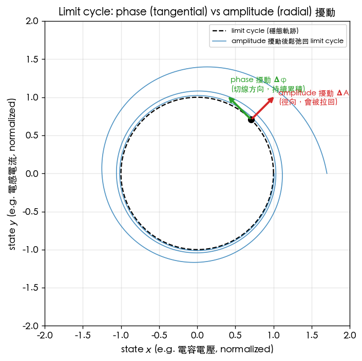
Physical intuition (2-D projection): an injected charge $\Delta q$ nudges the state point. Decompose the nudge along the two orthogonal directions of the limit cycle — tangential (phase, permanent) measured by $\Gamma$, radial (amplitude, pulled back) measured by $\Lambda$. Phase noise cares only about the tangential part; the full dynamics of injection need both.

Key equations

APF definition and amplitude decay function (verified against the original PDF ✓)

The APF $\tilde\Lambda$ is the amplitude analog of Part I's unit-bearing ISF $\tilde\Gamma=\Gamma/q_{max}$: the weight with which an injected current impulse projects onto the radial (amplitude) direction of the limit cycle. [P4] factors the amplitude perturbation into the product of an APF and a decay, $D(\tau,\phi)=\tilde\Lambda(\phi)\,d(\tau,\phi)$ ([P4] Eq.(18), p.2126), and defines the APF $\Delta(\phi):=\int_0^\infty D(\tau,\phi)\,d\tau$ ([P4] Eq.(19), p.2126, units $1/\text{A}$). Unlike phase, amplitude perturbations decay — the ideal-LC amplitude decay function (in the ideal-LC section, [P4] p.2127–2128) is:

$$d(t,\phi)=e^{-t/\tau_0},\qquad \int_0^\infty d(t,\phi)\,dt=\tau_0=\frac{2Q}{\omega_{osc}}$$

Key physics (gem): the "memory time" of the amplitude is $\tau_0=2Q/\omega_{osc}$ — a high-$Q$ LC recovers its amplitude slowly ($\tau_0$ is large), but it does recover (exponential decay back to the limit cycle); the phase has no such restoring force (its impulse response is a unit step — infinite memory). This is the quantitative version of "why amplitude noise is suppressed while phase noise accumulates" (claim C2). For an ideal LC, the APF and the decay are related by $\Delta(\phi)=\tau_0\,\tilde\Lambda(\phi)$.

Comparison table (ISF vs APF):

Quantity	Projection direction	Symbol	Fate of the perturbation
ISF	tangential (phase)	$\tilde\Gamma=\Gamma/q_{max}$	accumulates permanently (impulse response = unit step)
APF	radial (amplitude)	$\tilde\Lambda$	decays back to the limit cycle as $e^{-t/\tau_0}$, $\tau_0=2Q/\omega_{osc}$

Verified: the APF factorization $D(\tau,\phi)=\tilde\Lambda(\phi)\,d(\tau,\phi)$ ([P4] Eq.(18), p.2126), the APF definition $\Delta(\phi)=\int_0^\infty D\,d\tau$ ([P4] Eq.(19), p.2126, units $1/\text{A}$), and the ideal-LC decay function $e^{-t/\tau_0}$, $\tau_0=2Q/\omega_{osc}$ ([P4] ideal-LC section, p.2127–2128) have all been confirmed verbatim against the rendered original PDF.

Quadrature of the ISF and APF (ideal LC, verified ✓)

The ISF and APF fundamentals of an ideal LC ([P4] Eq.(26), p.2128):

$$\tilde\Gamma_1=\frac{1}{q_{max}}\,\angle 90^\circ,\qquad \tilde\Lambda_1=\frac{\tau_0}{q_{max}}\,\angle 0^\circ$$

Their phase difference is exactly $90^\circ$ (quadrature) (claim C11). Physical meaning: injecting at the zero-crossing changes almost purely phase ($\tilde\Gamma$ large, $\tilde\Lambda$ small); injecting at the peak changes almost purely amplitude ($\tilde\Lambda$ large, $\tilde\Gamma$ small). Note the APF fundamental carries an extra factor of $\tau_0$ relative to the ISF — at high $Q$ the amplitude effect ($\propto\tau_0=2Q/\omega_0$) is actually more pronounced, which is also why LC injection locking often comes with substantial amplitude modulation.

Amplitude-corrected Adler (augmented pulling, ideal-LC special case [P4] Eq.(27), p.2128): substitute the ISF and APF together. The general sinusoidal-injection form is [P4] Eq.(22), p.2126 (with a $+$ sign and phase-offset terms $\cos(\theta+\angle\tilde\Gamma_1)/\cos(\theta+\angle\tilde\Lambda_1)$); substituting the ideal-LC quadrature angles $\angle 90^\circ/\angle 0$ (Eq.(26)) into Eq.(22), the phase equation under sinusoidal injection simplifies to

$$\frac{d\theta}{dt}=(\omega_0-\omega_{inj})-\frac{\tfrac12\,(I_{inj}/q_{max})\sin\theta}{1+\tfrac12\,(I_{inj}\tau_0/q_{max})\cos\theta}$$

The denominator term is the amplitude-modulation correction contributed by the APF; Part I's phase-only Adler is the special case with denominator $=1$.

Verified: the quadrature of $\tilde\Gamma_1,\tilde\Lambda_1$ ([P4] Eq.(26), p.2128; sin/cos form in Eq.(24)) and the amplitude-corrected Adler shown above — i.e., the ideal-LC special case [P4] Eq.(27), p.2128 (obtained by substituting the $\angle 90^\circ/\angle 0$ of Eq.(26) into the general form Eq.(22), p.2126, with the $-$ sign, the $\sin\theta$ numerator, and the $\tau_0$ factor) — have both been confirmed verbatim against the rendered original PDF.

Amplitude modulation (the Fourier view of the APF)

Meaning: expanding the APF as a Fourier series, one can compute how the injection waveform is "filtered" into amplitude modulation ([P4] Sec. III-D text). For the concrete stage allocation and modulus switching, see [P4] Sec. VIII (dual-modulus prescaler, from p.2135; schematic Fig.19, Table VIII, and Fig.21 on p.2137).

The formal math of M:N sub-/super-harmonic locking and the ILFD ([P4] Sec. IV, Eq.(28)–(30), p.2129, verified ✓)

The generalized Adler of [P3] only handles $\omega_{inj}\approx\omega_0$. [P4] Sec. IV generalizes it to an arbitrary rational frequency ratio: under lock, $M\omega_{inj}=N\omega_{osc}$ ($M,N$ coprime positive integers). This is the math shared by the ILFD ($M=1$: output $=\omega_{inj}/N$, i.e., divide-by-$N$) and the injection-locked frequency multiplier ($N=1$: multiply-by-$M$). The whole derivation uses one move: time-synchronous averaging keeps only the single "resonant" ISF harmonic. Step by step:

Step 1 (re-define the relative phase, [P4] Eq.(28), p.2129):

$$\varphi(t)\equiv\frac{M}{N}\,\omega_{inj}t+\theta(t)$$

$\varphi$ is the oscillator's total phase [rad], and $\theta$ is the slowly varying phase relative to the injection clock [rad]. A ÷2 ILFD takes $M=1$, $N=2$: inject at $\omega_{inj}\approx2\omega_0$, and the oscillator runs at $\omega_{inj}/2$.

Step 2 (generalized pulling equation, [P4] Eq.(29), p.2129): substitute Eq.(28) into the instantaneous pulling equation (the same step as [P3] Eq.(28)–(29), p.2113, except $\omega_{inj}t$ becomes $(M/N)\,\omega_{inj}t$), then time-synchronously average over a window of $NT_{inj}$ (not $T_{inj}$):

$$\frac{d\theta}{dt}=\omega_0-\frac{M}{N}\omega_{inj}+\frac{1}{NT_{inj}}\int_{NT_{inj}}\tilde\Gamma\!\left(\frac{M}{N}\omega_{inj}t+\theta\right)i_{inj}(t)\,dt$$

Why a window of $NT_{inj}$? Within the window the injection waveform completes $N$ full cycles; the ISF argument advances by $(M/N)\,\omega_{inj}\cdot NT_{inj}=2\pi M$, i.e., $M$ full cycles. [P4] p.2129 says it explicitly: the framework does not require the fundamental period of the injection or the ISF to equal the averaging interval — "they need only iterate through an integer number of cycles over a single averaging period" — this is the linchpin of the whole M:N theory.

Step 3 (term-by-term averaging — only the resonant harmonic survives): take $M=1$ and a sinusoidal injection $i_{inj}=I_{inj}\cos(\omega_{inj}t)$ ($I_{inj}$ in A). Expand $\tilde\Gamma$ as a phasor Fourier series (the same expansion as [P1] Eq.(12); the correspondence is $\vert\tilde\Gamma_n\vert=c_n/q_{max}$, units rad/C):

$$\tilde\Gamma(\varphi)=\tilde\Gamma_{dc}+\sum_{n=1}^{\infty}\vert\tilde\Gamma_n\vert\cos\!\big(n\varphi+\angle\tilde\Gamma_n\big)$$

Multiply the $n$-th term by the injection and use the product-to-sum identity ($\cos A\cos B=\tfrac12[\cos(A-B)+\cos(A+B)]$):

$$\vert\tilde\Gamma_n\vert\cos\!\Big(\tfrac{n}{N}\omega_{inj}t+n\theta+\angle\tilde\Gamma_n\Big)\,I_{inj}\cos(\omega_{inj}t) =\frac{I_{inj}\vert\tilde\Gamma_n\vert}{2}\left[\cos\!\Big(\tfrac{n-N}{N}\omega_{inj}t+n\theta+\angle\tilde\Gamma_n\Big)+\cos\!\Big(\tfrac{n+N}{N}\omega_{inj}t+n\theta+\angle\tilde\Gamma_n\Big)\right]$$

Over the $NT_{inj}$ window, the difference-frequency term's phase advances by $2\pi(n-N)$ and the sum-frequency term's by $2\pi(n+N)$ — except for the $n=N$ difference-frequency term (whose frequency is exactly 0), every term completes an integer number of cycles and averages exactly to zero (this is an identity, not "approximately small"; lab_37 verifies it numerically to $10^{-15}$). The single surviving term is [P4] Eq.(30), p.2129:

$$\Omega(\theta)=\frac{1}{2}\,I_{inj}\,\vert\tilde\Gamma_N\vert\cos\!\big(N\theta+\angle\tilde\Gamma_N\big)$$

Factor-of-2 bookkeeping: this $\tfrac12$ is the product-to-sum $\tfrac12$ (two cosines multiplied, only the difference-frequency term survives), and has nothing to do with the SSB $/4$ vs time-domain $/2$ bookkeeping convention on the phase-noise pages (the 4 in [P1] Eq.(21)).

Step 4 (lock range and the $2\pi/N$ degeneracy): dimension check: $[\text{A}]\times[\text{rad/C}]=[\text{C/s}]\times[\text{rad/C}]=[\text{rad/s}]$ ✓. Locking = $d\theta/dt=0$ has a stable solution ⟺ $\vert\omega_{inj}/N-\omega_0\vert\le\max_\theta\Omega(\theta)$, so the half lock range ([P4] p.2130, verbatim: "which can be calculated from (30) to be $\omega_L=I_{inj}\vert\tilde\Gamma_N\vert/2$") is:

$$\omega_L=\frac{1}{2}\,I_{inj}\,\vert\tilde\Gamma_N\vert=\frac{I_{inj}\,c_N}{2\,q_{max}}$$

Three pieces of physics you can read off immediately:

1. The division ratio $N$ does not appear directly in the formula — it only selects which harmonic $c_N$ is used. The ÷2 lock range rides on $c_2$, and ÷3 rides on $c_3$ (lab_37 panel (b): the two measured datasets fall on one and the same $f_L\propto c_N$ line).
2. $\omega_L$ is reckoned on the output (oscillation) frequency axis ($\Delta\omega\equiv\omega_{inj}/N-\omega_0$, [P4] p.2130); converted to the injection-frequency axis, the lockable $\omega_{inj}$ window is $2N\omega_L$ wide.
3. The period of $\Omega(\theta)$ is $2\pi/N$ ⟹ there are $N$ stable locked phases spaced $2\pi/N$ apart that are mutually indistinguishable ([P4] p.2129, verbatim: "relative phases that are $2\pi/N$ apart are indistinguishable"). This is precisely the divider's well-known output phase ambiguity (a ÷$N$ output has $N$ possible phase startpoints), which must be handled separately in multi-phase/quadrature clocking.

Example (÷2 ILFD: 10 GHz in, 5 GHz out, canonical values): given $f_0=5$ GHz, $q_{max}=1$ pC, a sinusoidal injection of $I_{inj}=0.5$ mA at $f_{inj}\approx10$ GHz, and ISF second harmonic $c_2=0.5$.

1. $\vert\tilde\Gamma_2\vert=c_2/q_{max}=0.5/10^{-12}=5\times10^{11}$ rad/C.
2. $\omega_L=\tfrac12 I_{inj}\vert\tilde\Gamma_2\vert=\tfrac12\,(5\times10^{-4}\,\text{A})(5\times10^{11}\,\text{rad/C})=1.25\times10^{8}$ rad/s.
3. $f_L=\omega_L/2\pi=19.9$ MHz (only $0.40\%$ of $f_0$); the lockable window on the injection-frequency axis is $2Nf_L=79.6$ MHz wide (around 10 GHz).
4. Dimension check: A $\times$ rad/C = rad/s ✓. Weak-injection check: $I_{max}:=\omega_0 q_{max}=31.4$ mA ([P4] footnote 11, p.2130), $I_{inj}/I_{max}=1.6\%$ ⟹ the first-order linear model applies.

One-line Python verification: 0.5*0.5e-3*0.5/1e-12 → $1.25\times10^{8}$.

Payoff: a half-wave-symmetric ISF cannot divide by 2. Look back at the symmetry table in Step 7 of fourier_series_of_isf: half-wave symmetry $\Gamma(x+\pi)=-\Gamma(x)$ ⟹ the even harmonics $c_2=c_4=\cdots=0$. Substitute into $\omega_L=I_{inj}c_2/(2q_{max})$: the ÷2 lock range is identically zero — to first order, no matter how large you make $I_{inj}$, an injection at $2f_0$ simply will not lock. The same symmetry table that is good news on the phase-noise side (noise near $2\omega_0$ does not fold back onto the carrier) is bad news for the ILFD: symmetry is a double-edged sword. The design way out is to change the injection node — the ISF is "one curve per injection node" (as in [P1]): the differential output nodes have $c_2\approx0$ by symmetry, but the tail node already swings at $2f_0$, and the effective ISF seen from there has large even harmonics; [P4]'s ÷2 experiments inject $2f_0$ precisely into the tail of a differential LC (Fig. 11(a)(b) caption and Fig. 12(d), p.2130–2131, verified).

Transient and out-of-lock behavior ([P4] Eq.(31)–(34), p.2130, verified ✓): inside the lock range, the phase converges exponentially to the locked phase at the pull-in frequency $\omega_p=N\sqrt{\omega_L^2-\Delta\omega^2}$ (Eq.(32); Eq.(31) gives the closed-form tanh solution); outside, $\theta$ beats at the beat frequency $\omega_b=N\sqrt{\Delta\omega^2-\omega_L^2}$ (Eq.(34)) with an average drift rate of $\omega_b/N$, and the spectrum grows sidebands spaced $\omega_b$ apart — [P3]'s quasi-lock/pulling story replayed in its M:N version.

Applicability / failure conditions:

• First-order averaging requires weak injection ($I_{inj}\ll I_{max}=\omega_0 q_{max}$, [P4] footnote 11, p.2130) and $\omega_L\ll\omega_0$; strong injection needs the APF correction of the previous section (the denominator of Eq.(27)) and amplitude dynamics.
• $M\neq1$ (subharmonic injection, multipliers) requires the $M$-th harmonic of the injection signal — a sinusoidal injection has no harmonics, so in practice they are generated by mixing inside the oscillator; [P4] footnote 10, p.2129 states explicitly that this is not captured by the framework (partially addressed by the model of its reference [25]). This site turns the multiplier direction into its own page: assuming the injection waveform already carries the $N$-th harmonic (a pulse generator does exactly that), the multiplier closed form $\omega_L=\tfrac12\vert I_N\vert\vert\tilde\Gamma_1\vert$ follows directly from this page's Eq.(29) — see subharmonic_injection; the divider direction (this section's main line) has its full teaching page at injection_locked_division.
• "$c_2=0$ cannot divide by 2" is a first-order conclusion: higher-order mixing can still leave a tiny residual lock range (below lab_37's detection floor).

Experimental evidence ([P4] Fig. 12, p.2131, verified ✓): a Bose relaxation oscillator ($f_0=11.9$ MHz) at $N=2,3,4,5$; a 17-stage single-ended inverter-chain ring ($f_0=1.09$ GHz) at $N=2,5$; a 6-stage differential ring and an NMOS astable multivibrator at $N=3$; and a differential LC tail at $N=2$ — all measured lock ranges are linear in $I_{inj}$ with slopes set by $\vert\tilde\Gamma_N\vert$, matching the prediction of Eq.(30).

Numerical verification: lab_37 (unaveraged-ODE frequency sweeps + harmonic maps)

Integrate the unaveraged instantaneous equation directly (verifying Eq.(30) with the already-averaged Eq.(30) would be circular):

$$\frac{d\theta}{dt}=\Big(\omega_0-\frac{\omega_{inj}}{N}\Big)+\tilde\Gamma\!\Big(\frac{\omega_{inj}}{N}t+\theta\Big)\,I_{inj}\cos(\omega_{inj}t)$$

The ISF is a 3-harmonic toy (pedagogical toy, not transistor-level): $\tilde\Gamma(x)=-\big(c_1\sin x+c_2\sin2x+c_3\sin3x\big)/q_{max}$ (i.e., $\angle\tilde\Gamma_n=90^\circ$).

Parameter	Value	Units
$f_0$	5	GHz
$q_{max}$	1	pC
$I_{inj}$	0.5	mA
$(c_1,c_2,c_3)$	$(1.0,\,0.5,\,0.2)$	—
ODE step / total time	1 ps / 600 ns	—
Theory $f_L$ ($N=2$, $c_2=0.5$)	19.89	MHz
Theory $f_L$ ($N=3$, $c_3=0.2$)	7.96	MHz

PYTHONPATH=. python simulations/lab_37_ilfd_lock.py
# -> 1.13e-15 / 3.19e-15 (max relative error of the numerical average of Eq.(29) vs the closed form Eq.(30), N=2 / N=3: identity-level)
# -> 1.033 (2f0 sweep: measured omega_L / theory 1.25e8 rad/s; the 61-point grid resolves ~3%)
# -> 1.000 (3f0 sweep: measured omega_L / theory 5e7 rad/s)
# -> 0/61 (locked points of the half-wave-symmetric c2=0 ISF on the same ±2 omega_L grid: never locks, no ÷2)
# -> 1.004 / 1.019 (mean measured/theory ratio of the lock range swept vs c2 (N=2) and vs c3 (N=3): linearity holds)
# -> 1.000 (out-of-lock mean drift rate / (omega_b/N), [P4] Eq.(34))
# -> 3.1330 (difference between converged phases from two initial conditions at N=2, theory 2pi/2=3.1416: the 2pi/N degeneracy)

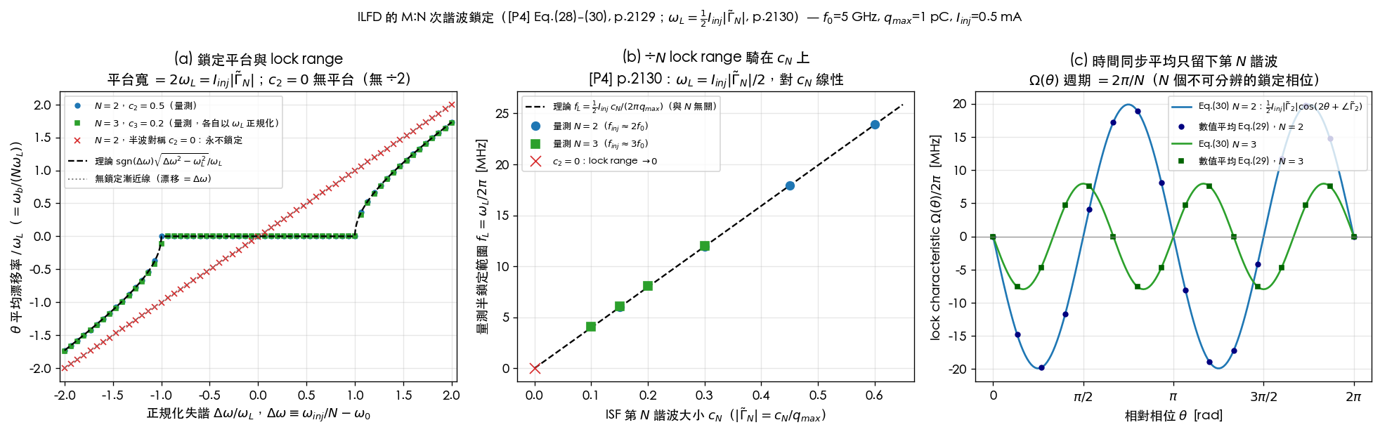
How to read it (full script: simulations/lab_37_ilfd_lock.py, runtime ≈ 19 s):

• (a): horizontal axis $\Delta\omega/\omega_L$, vertical axis the mean drift rate of $\theta$. Locking = the zero-drift plateau, whose half-width is exactly $\omega_L$; outside the plateau the measured points fall on the theory curve $\mathrm{sgn}(\Delta\omega)\sqrt{\Delta\omega^2-\omega_L^2}$ ($=\omega_b/N$, Eq.(34)). The red $c_2=0$ (half-wave-symmetric) curve is a straight line through the origin (drift = detuning): it never locks at any detuning.
• (b): measured half lock range plotted against $c_N$ — the $N=2$ and $N=3$ points fall on one and the same theory line $f_L=I_{inj}c_N/(4\pi q_{max})$ ($N$ only selects the harmonic; it does not enter the formula).
• (c): the averaging integral of Eq.(29) evaluated numerically for each $\theta$, overlapping the closed form Eq.(30); period $\pi$ for $N=2$ and $2\pi/3$ for $N=3$ — the $2\pi/N$ degeneracy visible to the naked eye.

Limitations: a first-order phase-only toy (no APF/amplitude dynamics, no noise); ISF harmonics only up to $n=3$; the lock-edge determination is limited by the 600 ns integration window and grid resolution (~1–3%).

Key figures

Paper figure	Page	Content	Teaching purpose
Fig. 5	2126	Characterizing the effect of an instantaneous charge injection on the oscillator: ISF / excess phase, the amplitude decay function, and the quadrature relation between ISF and APF (verified)	The single best figure connecting phase (ISF) and amplitude (APF) sensitivities
Fig. 11	2130	Superharmonic sinusoidal lock characteristic simulations: 1-mA and 2-mA second-harmonic injections into the tail of a differential LC ($I_{tail}=1$ mA), and a 5-mA third-harmonic injection into an ideal Bose oscillator (caption verified)	÷2/÷3 lock characteristics against Eq.(30); injecting at the tail for ÷2 bypasses the $c_2\approx0$ of the differential nodes
Fig. 12	2131	Superharmonic lock range measurements: Bose relaxation ($N=2..5$), 17-stage ring ($N=2,5$), various oscillators ($N=3$), differential LC tail ($N=2$) (caption verified)	Experimental verification of $\omega_L=I_{inj}\vert\tilde\Gamma_N\vert/2$: linear in $I_{inj}$

This figure is the best visual for "why amplitude noise decays while phase noise does not": the perturbation associated with the APF is pulled back by the amplitude decay function, whereas the phase perturbation associated with the ISF remains permanently. This site uses the same concept in phase_vs_amplitude_noise (toy comparison figure limit_cycle_phase_amplitude.png, not transistor-level).

Verified: this figure is [P4] Fig. 5, p.2126, captioned "Characterizing the effect that an instantaneous injection of charge has on an oscillator," confirmed against the rendered original PDF. (Fig. 3 p.2124 is the impulse-train↔sinusoid equivalence, and Fig. 6 p.2127 is the bipolar Colpitts example — neither is this figure.)

Design insights

• Strong injection / transients require the amplitude: ignoring the APF is fine for weak injection; for strong injection, transient locking, and frequency division, amplitude modulation cannot be ignored — compute with ISF + APF together.
• Quadrature is a design tool: to modulate phase purely, inject at the phase-sensitive point (ISF extremum); for amplitude keying / AM, inject at the amplitude-sensitive point (APF extremum).
• The ILFD is a low-power divider: compared with latch-based / CML dividers, which burn power at high frequency, the ILFD divides via injection locking at low power; use the $N$-th harmonic of the ISF/APF to design the division ratio and lock range.
• Dual-modulus prescaler: switch the division ratio on the same inverter-chain ring via a quadrature injection scheme, saving power.
• The large-injection / transient leftovers: Mirzaei's generalized Adler (Eq.(8)–(9)), the exact pull-in/pulling closed-form solutions (Eq.(31)–(34)), the APF-driven amplitude transient (dip→overshoot), and the full derivation and numerical verification of the large-injection pulling spectrum live in paper_004_large_injection_transient.

Limitations

Per paper_metadata (paper_004.limitations):

• Strongly nonlinear effects beyond the first-order APF are only partially captured; the injection harmonics required when $M\neq1$ are generated by internal mixing, which is outside the framework ([P4] footnote 10, p.2129).
• Relative to this site's core ISF phase-noise goal, it is advanced / peripheral.
• The exact APF equations ([P4] Eq.(18)–(22), p.2126; quadrature Eq.(26), p.2128) and the M:N locking (Eq.(28)–(30), p.2129; $\omega_L$, p.2130) have been verified against the original (claim C11).

Relationship to other papers

• [P3] is the direct prequel: this paper uses Part I's time-synchronous ISF model and adds amplitude (APF).
• [P1] provides the ISF $\Gamma$; the APF is its radial dual. The ideal-LC $\Gamma=-\sin$ also appears in this site's isf_definition.
• [P2] provides the ring ISF; the ILFD/prescaler in this paper is implemented with an inverter-chain ring.
• [P5] is unrelated to this page (sense amplifier); but the start-up of LC / latch oscillators likewise relies on cross-coupled positive feedback (the corner-case bridge of claim C12).
• The APF is entry 21 in equation_index (verified on this page against [P4] Eq.(18)–(22)); the phase/amplitude geometry is in phase_vs_amplitude_noise.

Further reading / corresponding teaching pages

Which part of this page	Corresponding teaching page	What that page adds
The ÷$N$ lock range rides on $c_N$; half-wave symmetry ⟹ $c_2=0$ cannot divide by 2	fourier_series_of_isf	ISF Fourier expansion, the Step-7 symmetry table (odd function ⟹ $c_0=0$; half-wave symmetry ⟹ even harmonics vanish)
Injection phase sets the effective weight of $\Gamma$ / $\Lambda$ (cyclostationary concept)	effective_isf	$\Gamma_{eff}=\Gamma\cdot\alpha$, bias-dependent thermal-noise NMF, switching-pair worked example
How injection phase changes the effective ISF (numerical feel)	lab_14_cyclostationary_isf	Runnable toy: noise injection phase $\to$ $\Gamma_{eff,rms}$ (pedagogical toy, not transistor-level)
ISF / APF quadrature, coupled oscillators under injection locking	quadrature_and_coupled_oscillators	Quadrature injection, phase relations and design of coupled oscillators

How to read: this page completes the phase framework of [P3] into phase + amplitude. To understand "why the injection phase (or noise injection phase) changes the effective sensitivity," effective_isf and lab_14 are the theory and hands-on versions of the same cyclostationary concept; to see how quadrature becomes a usable design tool, return to quadrature_and_coupled_oscillators. For the phase/amplitude geometry, also see phase_vs_amplitude_noise.

What to remember

• APF = the amplitude version of the ISF, units $1/\text{A}$; the ISF projects onto the tangential direction (phase), the APF onto the radial direction (amplitude).
• Ideal LC: the ISF and APF are in quadrature ($90°$ apart) — when phase is most sensitive, amplitude is least sensitive, and vice versa (claim C11).
• Phase accumulates permanently; amplitude is pulled back by the decay function — this is the justification for "tracking only phase" in phase noise.
• ILFD: inject at $\omega_{inj}\approx N\omega_0$ and lock to $\omega_{inj}/N$ via the $N$-th ISF harmonic; the half lock range is $\omega_L=\tfrac12 I_{inj}\vert\tilde\Gamma_N\vert=I_{inj}c_N/(2q_{max})$ ([P4] Eq.(30) p.2129 and p.2130); $N$ only selects the harmonic and does not enter the formula; the output has $N$ indistinguishable locked phases spaced $2\pi/N$ apart.
• A half-wave-symmetric ISF ($c_2=0$) cannot divide by 2 to first order — the symmetry that is good for phase noise is bad news for the ILFD; [P4]'s ÷2 experiments inject $2f_0$ into the tail of a differential LC to get around it.
• This page is advanced; the exact APF equations ([P4] Eq.(18)–(22), p.2126; quadrature Eq.(26), p.2128) and the M:N locking (Eq.(28)–(30), p.2129; $\omega_L$, p.2130) have been verified against the original.