β: This English translation is in beta — the Traditional-Chinese original is the authoritative version.

Lab 40 — Subharmonic (×N) Pulse Injection: Impulse-Train Map vs. Unaveraged Time-Synchronous ODE

Prerequisites: subharmonic_injection (every closed form this lab verifies — the lock range, the realignment factor $\beta$, discrete-time noise shaping, output jitter, and the reference spur), paper_003 ([P3] Sec. IV's impulse train and footnote 7's subharmonic arithmetic), paper_004 ([P4] Eq.(28)–(30)'s M:N averaging equation) | Next: injection_locked_division (the dual, divider direction), sampling_pll, clock_chain_budget

The subharmonic_injection page has already derived every formula for the injection-locked clock multiplier (ILCM) step by step: the multiplier closed form $\omega_L=\tfrac12\vert I_N\vert\vert\tilde\Gamma_1\vert$ from [P4] Eq.(29), the $\Delta\omega_L\propto1/N$ scaling from the discrete arithmetic of [P3] footnote 7, the realignment factor $\beta$ from the linearized per-pulse map, and the output-jitter closed form from putting noise on a first-order discrete loop. This page does not re-derive any of it — it uses two independent numerical engines to score every one of those closed forms term by term.

What this lab verifies:

1. Does the lock range really go as $1/N$ (Engine 2: sweep $N$ with the unaveraged ODE)?
2. How does a finite pulse width eat into the lock range — a clean sinc for LC, and what about the ring (Engine 2: sweep the pulse width)?
3. At the same rms current, does the pulse train really lock while a pure sine really doesn't (Engine 2: pulse-train vs. sine comparison)?
4. How accurate is the first-order prediction $-q_{inj}\tilde\Gamma'(\theta_{ss})$ for the realignment factor $\beta$ (Engine 2: step response)?
5. Is the locked phase noise really a first-order discrete high-pass, with corner $\approx\beta f_{ref}/2\pi$ (Engine 1: map + white FM noise)?
6. Does output jitter really go as $\sqrt N$, and is the reference spur really independent of $\beta$ (Engine 1: edge-level simulation)?

Physical intuition: the two engines measure the same physics at different resolutions. Engine 1 (the map) compresses one pulse's effect into an instantaneous jump $\theta_{k+1}=\theta_k+\Delta\omega_0NT_0+q_{inj}\tilde\Gamma(\theta_k)+n_k$ — fast, well suited to long-horizon noise statistics (PSD, jitter), but assumes the pulse is narrow. Engine 2 (the unaveraged ODE) honestly integrates the instantaneous equation $\dot\theta=\Delta\omega+\tilde\Gamma(N\omega_{inj}t+\theta)(q_{inj}/\tau_p)$ through the pulse with RK4 — it sees pulse-width effects and $\beta$'s second-order correction (the phase is already moving during the pulse), but each data point costs thousands of periods of integration, so it is best suited to "does it lock or not" edge sweeps. The two engines agree to within 0.1%–1% at the canonical parameters — that agreement is this lab's acceptance criterion.

Where this page sits: an independent verification lab. All the theory has already been derived step by step, with sources flagged ([P3]/[P4] verified portions vs. this site's own derivations vs. external literature), on subharmonic_injection; this page lists only the verification core code and the resulting numbers. Pedagogical toy model: phase-only, weak injection, no transistors.

---

1. Learning goals

• Independently verify $\text{lock range}\propto1/N$ using the unaveraged time-synchronous ODE (not the already-averaged map) — this avoids the circular-reasoning trap of "verifying an averaged formula with the same averaged formula" (log-log slope $-1.000$, for both LC and ring).
• Sweep the pulse width $\tau_p$: LC's lock range follows $\mathrm{sinc}(\tau_p/T_0)$ exactly (a single harmonic, max deviation $10^{-4}$); the ring's sharp ISF spreads its energy across multiple harmonics, so a plain sinc is not enough (deviation up to 0.74) — only a "box-averaged whole ISF" matches (deviation $\le0.0074$).
• At equal rms current, the pulse train locks throughout the lock range (15/15 grid points) while a pure sine cannot lock at first order anywhere (0/15) — pinning down numerically what subharmonic_injection Section 1 states in words: "a pure sine cannot lock."
• The realignment factor $\beta$'s ODE step response against the first-order prediction $-q_{inj}\tilde\Gamma'(\theta_{ss})/q_{max}$: ratio $0.98$–$1.03$ ($q_{inj}/q_{max}=0.05$), tightening to $0.995$–$1.03$ at $q_{inj}/q_{max}=0.01$ — the deviation is a second-order, $O(q_{inj}/q_{max})$ effect (the phase is already moving during the pulse), matching the precision the linear theory promises.
• Put white FM noise on the map and measure the locked phase's PSD: the low-frequency plateau matches theory to a ratio of $0.991$, and the corner measures $1.934$ MHz (simplified theory $1.981$ MHz; the exact discrete closed form gives $1.934$ MHz — the measurement rides right on the exact form).
• Edge-level simulation of the output jitter's power law in $N$: fitted slope $0.497$ (theory $0.5$); the canonical $N=20$ gives $2.226$ fs (closed form $2.228$ fs).
• The reference spur at a detuned lock: $k=1$ error $0.00$ dB, $k=2$ error $0.01$ dB — the first-order sawtooth approximation is nearly exact at the canonical parameters.

2. Mathematical model (the two engines and notation; full derivation on subharmonic_injection)

2.1 Engine 1: the linearized impulse-train map

$$\theta_{k+1}=\theta_k+\Delta\omega_0\,NT_0+\frac{q_{inj}}{q_{max}}\,\bar\Gamma(\theta_k)+n_k,\qquad n_k\sim\mathcal N(0,\kappa^2T_{inj})$$

$\bar\Gamma$ is the ISF box-averaged over the pulse width (the $k$-th harmonic multiplied by $\mathrm{sinc}(k\tau_p/T_0)$, reducing to $\Gamma$ in the impulse limit); $\kappa^2=0.125$ rad²/s is the canonical white-FM variance-growth rate (see diffusion_dictionary). Linearizing gives the realignment factor $\beta\equiv-\dfrac{q_{inj}}{q_{max}}\bar\Gamma'(\theta_{ss})$, corner $\omega_c=\beta/T_{inj}$, and the first-order discrete noise-shaping transfer functions $H_{ref}(z)=\dfrac{\beta}{1-(1-\beta)z^{-1}}$, $H_{osc}(z)=\dfrac{1-z^{-1}}{1-(1-\beta)z^{-1}}$.

2.2 Engine 2: the unaveraged time-synchronous ODE

$$\frac{d\theta}{dt}=\Delta\omega+\tilde\Gamma\big(N\omega_{inj}t+\theta\big)\,i_{inj}(t),\qquad i_{inj}(t)=\begin{cases}q_{inj}/\tau_p,&\vert t-kT_{inj}\vert<\tau_p/2\\0,&\text{otherwise}\end{cases}$$

RK4 is used during the pulse (with the number of sub-steps set by the ISF's curvature: LC at $\le0.2$ rad per sub-step, the ring's sharp triangle kinks at $\le0.05$–$0.08$ rad per sub-step, checked against a 512-sub-step reference to $\le0.4\%$/$0.85\%$ error); between pulses, $\dot\theta=\Delta\omega$ is skipped over analytically. "Does it lock" is read directly off the net correction of the lock characteristic $J(\theta)=\theta_{\text{after pulse}}-\theta_{\text{before pulse}}$ (a single integration at $\Delta\omega=0$) giving the edges $A_\pm=\mp\min/\max J(\theta)$, or cross-checked with a long-time convergence test (2500–4000 periods; locked $\Leftrightarrow$ the last 800–1300 periods satisfy $\vert\theta(\text{end})-\theta(\text{end}-n_{tail})\vert<5\times10^{-3}$).

2.3 Two toy ISFs (shared with other labs on this site)

$$\Gamma_{LC}(\theta)=-\sin\theta,\qquad \Gamma_{ring}(\theta)=\text{[P2] App.B triangular pulses (}\eta=0.75,\ N_{st}=17\text{, the same construction as lab\_39)}$$

The ring toy is two opposite-sign triangular pulses, height = half-width $=1/f'$ ($f'=\eta N_{st}/\pi=4.0585$ 1/rad), $\max\vert\Gamma_{ring}\vert=1/f'=0.2464$ — a pedagogical toy, not transistor-level.

2.4 Applicability and failure conditions

Condition	When it holds	What happens when it fails
Weak injection $q_{inj}\ll q_{max}$	Engine 1 linearizes correctly; $\beta$'s first-order prediction is accurate	Large injection: the $\beta$ ODE/map ratio deviates systematically from 1 (measured at $O(q_{inj}/q_{max})$ in (d))
Pulse width $\ll T_0$	$\bar\Gamma\approx\Gamma$; Engines 1 and 2 agree	$\tau_p\to T_0$: LC's lock range collapses to 0 (the null seen in (b))
$\theta$ varies slowly within $T_{inj}$	The two engines reconcile with each other	Near the lock-range edge: critical slowing, requiring more periods for the long-time convergence test
White-FM noise drive (Engine 1's noise part)	$\sigma_w^2=\kappa^2T_{inj}$; the PSD closed form holds	Flicker FM: not covered by this lab

---

3. Block diagram

4. Core Python code

Excerpted from simulations/lab_40_subharmonic_injection.py (checked against the source). The box-averaged table, the per-pulse map, and one pulse period of the unaveraged ODE (RK4):

def isf_tables(gamma_func, tp):
    """Gbar(theta) = ISF box-averaged over the pulse (width tp/T0), via FFT:
    k-th harmonic multiplied by sinc(k*tp/T0)."""
    g = gamma_func(XG)
    G = np.fft.rfft(g)
    k = np.arange(G.size)
    Gb = G * np.sinc(k * tp)
    gbar = np.fft.irfft(Gb, NG)
    gbar_p = np.fft.irfft(1j * k * Gb, NG)          # d Gbar / d theta
    return gbar, gbar_p

def pulse_period_step(theta, dw, n_div, qt, gamma_func, tp, nsub):
    """ENGINE 2: one injection period T_inj = n_div*T0 of the UNAVERAGED ODE —
    RK4 through the rectangular pulse (width tp), analytic free-run in between."""
    h = tp / nsub
    amp = qt / tp
    t = -tp / 2.0
    for _ in range(nsub):
        k1 = dw + amp * gamma_func(TWO_PI * t + theta)
        k2 = dw + amp * gamma_func(TWO_PI * (t + 0.5 * h) + theta + 0.5 * h * k1)
        k3 = dw + amp * gamma_func(TWO_PI * (t + 0.5 * h) + theta + 0.5 * h * k2)
        k4 = dw + amp * gamma_func(TWO_PI * (t + h) + theta + h * k3)
        theta = theta + (h / 6.0) * (k1 + 2 * k2 + 2 * k3 + k4)
        t += h
    return theta + dw * (n_div - tp)

def gbar_prime_exact(gamma_func, theta, tp):
    """Exact derivative of the box-averaged ISF (difference of raw Gamma at the
    two box ends over the box width) -- used for beta = -q_t * Gbar'(theta*)."""
    half_w = np.pi * tp
    return (gamma_func(theta + half_w) - gamma_func(theta - half_w)) / (2.0 * half_w)

Numbers printed by the script (PYTHONPATH=. python3 simulations/lab_40_subharmonic_injection.py, about 35 s single core; seed fixed with default_rng(40), results reproducible):

print(A_edge_pred['LC'])                    # -> 0.04979 rad/period (qt*max|Gbar|, N=20)
print(fL_pred['LC']/1e6)                    # -> 1.9813 MHz (with the 10 ps pulse-width sinc correction)
print(slope_N['LC'], slope_N['ring'])       # -> -1.000 -1.000 ((a) log-log slope, theory -1)
print(ratio_N['LC'].min(), ratio_N['LC'].max())   # -> 1.0000 1.0000 (LC measured/theory)
print(dev_lc_sinc)                          # -> 0.0001 ((b) LC: max deviation of ODE/f_L(0) from sinc)
print(dev_ring_box, dev_ring_sinc)          # -> 0.0074 0.7434 (ring: box average correct, plain sinc wrong)
print(n_lock_pulse, n_plateau_sine)         # -> 15 0 ((c): 15/15 grid points lock for the LC pulse train, 0 for the pure sine)
print(beta_c_lc[5], beta_c_lc[4])           # -> 0.04858 0.04979 ((d) headline beta: ODE vs. first order)
print(r_plateau, fc_meas/1e6, fc_pred/1e6)  # -> 0.991 1.9343 1.9813 ((e) plateau ratio, measured/theory corner)
print(slope_j, sig_all[10]/(2*np.pi*5e9)*1e15)  # -> 0.497 2.226 ((f1) jitter's power law in N, N=20 output in fs)
print(round(spur1[0], 2))                   # -> -67.96 ((f2) reference spur at 100 kHz detuning, dBc)

5. Full script path

simulations/lab_40_subharmonic_injection.py (depends on savefig from simulations/common/plot_utils.py and gamma_lc_ideal from simulations/common/isf_utils.py; uses scipy.signal.welch for the PSD and scipy.optimize.brentq to solve the exact discrete corner).

To run: PYTHONPATH=. python3 simulations/lab_40_subharmonic_injection.py (about 35 s single core; seed fixed with default_rng(40)).

6. Parameter table

Parameter	Program variable	Value	Meaning
Carrier	F0	5 GHz	canonical $f_0$
$q_{max}$	QMAX	1 pC	canonical
$q_{inj}$	QINJ	50 fC	charge per pulse ($q_{inj}/q_{max}=0.05$)
Pulse width	TAUP	10 ps	$\tau_p/T_0=0.05$
Multiplication ratio	N_HEAD	20	$f_{ref}=250$ MHz, $T_{inj}=4$ ns
$N$ sweep ((a))	N_list	2, 4, 8, 16, 20	lock range vs. $N$
Pulse-width sweep ((b))	tp_list	2–175 ps (9 points)	lock range vs. $\tau_p$
Detuning sweep ((c))	r_grid	$-1.5$–$1.5$ (25 points, $\times\omega_L/N$)	pulse-train vs. pure-sine drift curves
$q_{inj}/q_{max}$ ((d))	qt_arr	0.05, 0.01	two injection strengths for the $\beta$ step response
$\kappa^2$	KAPPA2	0.125 rad²/s	canonical (diffusion_dictionary)
PSD samples ((e))	K_PSD/M_W	$2^{18}$/32 walkers	Welch, nperseg$=2^{14}$
Edge-level samples ((f1))	K (depends on $N$)	$\ge4096$, 8 walkers	rerun per $N$
Ring toy	ETA, NST	0.75, 17	[P2] App.B construction, same as lab_39

7. Units table

Quantity	Symbol	Units
Phase	$\theta$	rad
Half lock range	$\omega_L$, $f_L$	rad/s, Hz
Realignment factor	$\beta$	dimensionless
Noise corner	$\omega_c$, $f_c$	rad/s, Hz
White-noise variance growth rate	$\kappa^2$	rad²/s
Phase PSD	$S(f)$	rad²/Hz
Output jitter	$\sigma_t$	s (fs)
Reference spur	—	dBc

8. Simulation figure

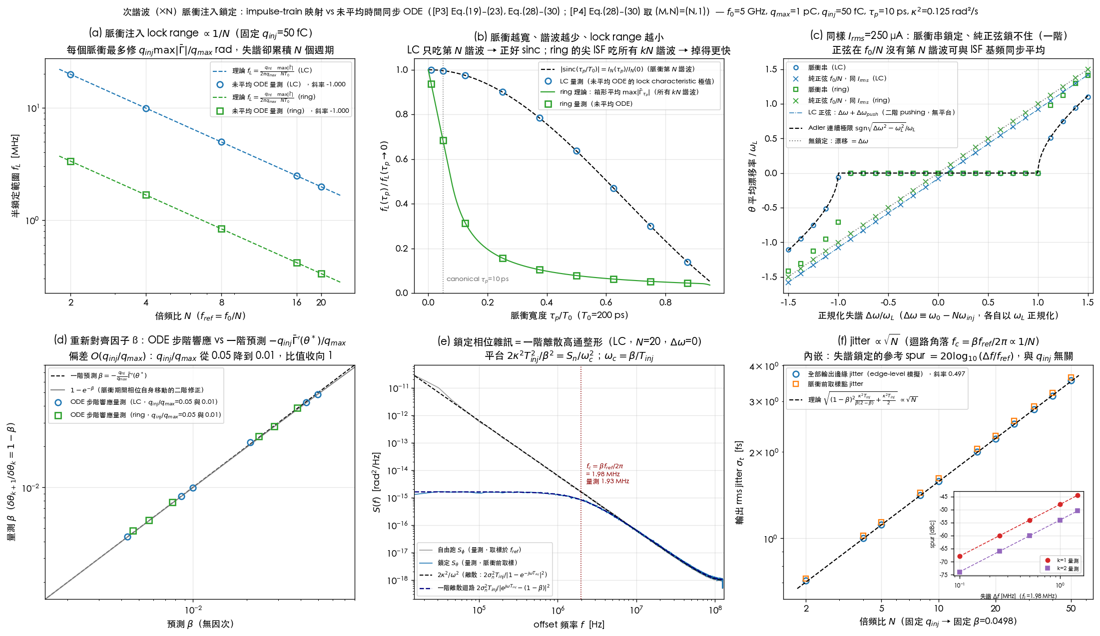
9. How to read the figure

(a) Lock range vs. $N$: the two theory dashed lines (LC, ring) are $f_L=\dfrac{q_{inj}}{2\pi q_{max}}\dfrac{\max\vert\bar\Gamma\vert}{NT_0}$; the circles/squares are the unaveraged-ODE measurements at $N=2,4,8,16,20$ — LC lies exactly on the theory line (ratio $1.0000$), the ring runs $0.30\%$ high (a slightly larger finite-pulse effect at the triangle's sharp corner). Both log-log slopes are $-1.000$: the same pulse has to pay for $N$-times-longer drift, no exceptions to the $1/N$ law.

(b) Lock range vs. pulse width: the black dashed line is the "plain sinc" reference (the decay of the single $k=N$ harmonic). LC's blue measured points lie exactly on that line (max deviation $10^{-4}$) — because LC's ISF has only one harmonic ($-\sin$), and locking taps only the $N$-th harmonic. The ring's green measured points fall off much faster and clearly deviate from the plain sinc (deviation up to $0.74$): the ring's triangular pulse spreads its energy across many harmonics ($m=1,2,3,\dots$, each paired with $mN$), and the pulse's box window shaves all of them at once — so only "box-average the whole ISF, then take the extremum" (the green solid line) matches the measurement (deviation $\le0.0074$). This is direct numerical evidence that a plain sinc is not enough for the ring.

(c) Pulse train vs. pure sine: the horizontal axis is the normalized detuning $\Delta\omega/\omega_L$. The pulse train (circles/squares) has its drift rate pinned at zero for $\vert x\vert<1$ (the locked plateau); the pure sine at the same rms current (crosses) has no plateau at all, only a line lightly offset by a second-order pushing effect (LC's fitted intercept $-0.0801\,\omega_L=-158.7$ kHz matches the analytic pushing formula $-(I/q_{max})^2\omega_0/(4(\omega_0^2-\omega_{inj}^2))$ to a ratio of $1.000$). The gray dashed line is the Adler continuous-limit beat frequency $\mathrm{sgn}\sqrt{(\Delta\omega/\omega_L)^2-1}$ — the pulse train's out-of-lock drift rate tracks it exactly (median ratio $1.001$). This figure is the most direct visual evidence that a pure sine cannot lock.

(d) $\beta$ step response: the black dashed line is the first-order prediction $\beta=-q_{inj}\bar\Gamma'(\theta^*)/q_{max}$; the gray solid line is $1-e^{-\beta}$ (the second-order correction from the phase moving during the pulse itself — the unaveraged ODE's exponential step essentially measures $1-e^{-\beta_{map}}$, not $\beta_{map}$ itself). Both LC and ring's measured points, at the two strengths $q_{inj}/q_{max}=0.05$ and $0.01$, sit on the gray line; comparing against the first-order prediction itself, LC's center-point ratio $0.9755$ matches $1-\beta/2=0.9751$ almost exactly — precisely "the first term of the second-order correction." This is a direct demonstration that the $\beta$ first-order theory's precision is $O(q_{inj}/q_{max})$.

(e) PSD: the gray line is the measured free-running $S_\phi$ (tracking the discrete version of $2\kappa^2/\omega^2$, ratio $0.999$), the blue line is the measured locked PSD, and the black dashed line is the first-order discrete theory $2\sigma_n^2T_{inj}/\vert e^{j\omega T_{inj}}-(1-\beta)\vert^2$. The low-frequency plateau ($1.613\times10^{-15}$ rad²/Hz) matches theory to a ratio of $0.991$; the red vertical line marks the corner, measured at $1.934$ MHz against the simplified prediction $\beta f_{ref}/2\pi=1.981$ MHz (a $2.4\%$ difference) — but against the exact discrete closed form $f_c'=\frac{f_{ref}}{2\pi}\arccos(1-\beta^2/(2(1+\beta)))=1.934$ MHz it is almost a perfect match (ratio $1.0002$). The simplified formula's $2.4\%$ gap is the known $O(\beta)$ correction, not a model error.

(f) Output jitter and spur: the main panel's circles are the edge-level simulation's full output-edge jitter at fixed $\beta$ (i.e., fixed $q_{inj}$) across different $N$; the black dashed line is the closed form $\sqrt{\kappa^2NT_0[(1-\beta)^2/(\beta(2-\beta))+1/2]}$; the fitted slope is $0.497$ against the theoretical $0.5$ — $\sigma_t\propto\sqrt N$ holds, giving $2.226$ fs at $N=20$ (closed form $2.228$ fs). The inset shows the reference spur at a detuned lock: the $k=1$ and $k=2$ measured points track $20\log_{10}(\Delta f_0/(kf_{ref}))$ exactly (max error $0.00$/$0.01$ dB) — the spur is a first-order, deterministic effect, independent of $\beta$.

10. Corresponding paper equations / figures

• [P3] Sec. IV footnote 7, p.2112 (verified): the injection can also land once every $M$ periods — this lab's impulse-train map (Engine 1) and the (a)(b) unaveraged-ODE lock-range sweeps are exactly this sentence's discrete arithmetic and its numerical verification.
• [P4] Eq.(28)–(30), p.2129 (verified): the $M{:}N$ time-synchronous averaging equation; this lab takes $(M,N)_{[P4]}=(N,1)$, whose term-by-term derivation into the multiplier closed form is written out in full on subharmonic_injection, Section 1 — this lab independently verifies that conclusion with Engine 2's unaveraged ODE (avoiding circular reasoning).
• [P4] footnote 10, p.2129 (verified): the injection harmonics needed for $M\neq1$ are "not explicitly captured by our framework" — this lab's (c) "pure sine 0/15 vs. pulse train 15/15" is exactly the numerical demonstration of that sentence: assuming the injection already carries the $N$-th harmonic (a pulse), the first-order theory applies directly.
• Noise shaping and the closed-form output jitter: derived on this site (not in the 5 PDFs); the full derivation is in Section 4 of subharmonic_injection, and this lab's (e)(f1) are that derivation's independent numerical adjudication.
• The first-order sawtooth reference-spur formula: derived on this site (subharmonic_injection, Section 4.4); this lab's (f2) verifies it via an FFT of the deterministic sawtooth phase modulation.

11. Limitations and approximations

• Phase-only toy model: amplitude dynamics (the APF) are ignored; at zero detuning the LC's lock point sits at the voltage peak, where a pulse also kicks the amplitude ([P4]'s APF), a second-order effect when $q_{inj}\ll q_{max}$ — not covered by this lab.
• Weak injection: $q_{inj}/q_{max}=0.05$ or $0.01$; (d) already measures the first-order theory's $O(q_{inj}/q_{max})$ deviation; stronger injection needs the APF correction from paper_004_large_injection_transient.
• White-FM noise assumption (Engine 1's noise part): $\sigma_w^2=\kappa^2T_{inj}$ is the exact result for white FM noise; under flicker FM the variance is no longer $\propto t$ — not covered by this lab.
• The ring toy is a triangular construction: a real ring's ISF flank is not a strict triangle, and its dead zone is not strictly zero; the order-of-magnitude conclusion driven by $q_{max}$ (the ring's $\beta$ wins on small $q_{max}$, not on slope) is unaffected by this simplification — see the ring-vs-LC table in Section 3 of subharmonic_injection.
• $f\ll f_{ref}/2$: (e)'s discrete $\vert H\vert^2$ equals the continuous first-order PLL only well below $f_{ref}/2$; sampling effects start to show up near $f_{ref}/2$ (this lab logs only near $f<f_{ref}/8$).
• First-order spur: (f2)'s sawtooth approximation ignores direct pulse feedthrough, AM caused by the APF, and pulse-width effects — none of these are in the phase-only model, and are honestly left out (see Section 4.4 of subharmonic_injection).

Key takeaways

• (a) Lock range $\propto1/N$: the unaveraged-ODE sweep over $N=2$–$20$ gives a log-log slope of $-1.000$ (LC and ring alike), with measured/theory ratios of $1.0000$ (LC) and $1.0030$ (ring).
• (b) Pulse-width effect: LC follows $\mathrm{sinc}(\tau_p/T_0)$ exactly (deviation $10^{-4}$); the ring's multi-harmonic energy makes the plain sinc fail (deviation $0.74$), requiring the extremum of the box-averaged ISF to match (deviation $0.0074$).
• (c) A pure sine cannot lock: at the same $I_{rms}=250\ \mu$A, the pulse train locks at 15/15 grid points while the pure sine locks at 0/15 — completely unable to lock at first order, with only the second-order pushing effect left (LC: $-158.7$ kHz, matching the analytic formula at a ratio of $1.000$).
• (d) $\beta$'s first-order precision: the ODE step response against the first-order prediction has ratio $0.98$–$1.03$ ($q_{inj}/q_{max}=0.05$), tightening at $0.01$; the deviation is essentially the second-order term $1-e^{-\beta}$, with headline $\beta_{ODE}=0.04858$ against the first-order $0.04979$.
• (e) Noise shaping: the locked PSD's low-frequency plateau matches theory to a ratio of $0.991$, and the corner measures $1.934$ MHz — an almost exact match (ratio $1.0002$) against the exact discrete closed form (not the simplified $\beta f_{ref}/2\pi$).
• (f) Jitter and spur: the output jitter's fitted power-law slope is $0.497\approx1/2$, giving $2.226$ fs at $N=20$ (closed form $2.228$ fs); the reference spur matches the first-order sawtooth formula to within $0.01$ dB.
• The two independent engines (the linearized map and the unaveraged ODE) agree with each other to within $0.1$–$1\%$ at the canonical parameters — every closed form on subharmonic_injection has passed this lab's numerical adjudication.

Further reading

• The full theoretical derivation this lab verifies: subharmonic_injection
• The impulse-train thought experiment and the subharmonic footnote: paper_003 ([P3] Sec. IV, p.2112)
• The original source of the M:N averaging equation: paper_004 ([P4] Eq.(28)–(30), p.2129)
• The dual, divider direction (÷N ILFD): injection_locked_division
• The source of $\kappa^2$ and its five outfits: diffusion_dictionary
• The continuous-time version of "a locked oscillator is a first-order PLL": injection_locking_noise
• Wiring the ILCM back into system-level accounting: clock_chain_budget, sampling_pll