Lab 16 — Leeson Model vs ISF Model (Three-Region Comparison)

Breadcrumb: Simulation labs › System & advanced › This page (Leeson vs ISF). Upstream: lab_06, lab_07; related: lab_09.

β: This English translation is in beta — the Traditional-Chinese original is the authoritative version.

The phase-noise model designers see most often actually comes in two lineages. One is Leeson (1966), an empirical formula: it fits a measured curve after the fact into three regions — $1/f^3$, $1/f^2$, and a flat floor — with parameters (quality factor $Q$, noise figure $F$, flicker corner) mostly obtained by fitting. The other is the ISF model, the main thread of this site: from [P1] Hajimiri–Lee's LTV theory it derives from first principles the same three regions, and every parameter has a physical origin ($\Gamma_{rms}$, $q_{max}$, $c_0$). This lab overlays the two curves on one plot so you can see clearly: they are two maps of the same mountain — Leeson describes "what it looks like", the ISF explains "why it looks that way".

External-literature note: the Leeson model is external literature, not among the five source PDFs; it is supplemented from the standard reference (D. B. Leeson, "A simple model of feedback oscillator noise spectrum," Proc. IEEE, 1966). This site treats it as a comparison baseline and historical context; the ISF model is the main thread. Step-by-step Leeson derivation and term-by-term comparison: see the appendix derivation_leeson.

Physical intuition (conclusion first): every free-running oscillator's phase noise looks the same from near to far — close to the carrier it is $1/f^3$ (flicker upconversion, steepest, $-30$ dB/dec), the middle is $1/f^2$ (white noise, $-20$ dB/dec), and the far end is a flat measurement/buffer floor. Leeson assembles the three regions with $Q$ and a corner; the ISF tells you the $1/f^2$ region's height is $\Gamma_{rms}^2/q_{max}^2$, the $1/f^3$ region is set by $c_0^2$, and the corner does not equal the device $1/f$ corner.

1. Learning objectives

• Recognize the three-region structure of the empirical Leeson model and its fitting parameters ($F,Q,$ flicker corner).
• Write the ISF model ([P1] Eq.(21) + Eq.(23) + floor) as the same three regions and overlay the plots.
• Understand the correspondence and differences of the two models in the $1/f^3$, $1/f^2$, and floor regions.
• Understand how the ISF gives Leeson's parameters physical meaning (and honestly flag Leeson as external literature).

2. Mathematical model

Leeson model (external literature, not among the five PDFs; verbatim per spec section 10.2):

$$\mathcal{L}(\Delta\omega)=10\log_{10}\!\left[\frac{2FkT}{P_s}\left(1+\Big(\frac{\omega_0}{2Q\Delta\omega}\Big)^2\right)\left(1+\frac{\omega_{1/f^3}}{\lvert\Delta\omega\rvert}\right)\right]$$

• First bracket $\big(1+(\omega_0/2Q\Delta\omega)^2\big)$: approaches $1$ at large offset (floor), and gives the $1/\Delta\omega^2$-shaped $1/f^2$ region at small offset; the corner is set by $Q$ (tank quality factor).
• Second bracket $\big(1+\omega_{1/f^3}/\vert\Delta\omega\vert\big)$: inside the corner it multiplies in an extra $1/\vert\Delta\omega\vert$, lifting $1/f^2$ into $1/f^3$.
• $F$ is the noise figure, $P_s$ the signal power, $kT$ the thermal noise — in Leeson these are mostly fitted/estimated values.

ISF model (derived from [P1] plus one white-noise floor): add the $1/f^2$ ([P1] Eq.(21)) and $1/f^3$ ([P1] Eq.(23)) regions on a linear scale, then add the floor:

$$\mathcal{L}(\Delta\omega)=10\log_{10}\!\left[\underbrace{\frac{\Gamma_{rms}^2}{q_{max}^2}\frac{\overline{i_n^2}/\Delta f}{4\,\Delta\omega^2}}_{1/f^2,\ \text{Eq.(21)}}+\underbrace{\frac{c_0^2}{q_{max}^2}\frac{\overline{i_n^2}/\Delta f}{8\,\Delta\omega^2}\frac{\omega_{1/f}}{\Delta\omega}}_{1/f^3,\ \text{Eq.(23)}}+\underbrace{\text{floor}}_{\text{flat}}\right]$$

• Physical correspondence: the ISF's $1/f^2$ region height $=\Gamma_{rms}^2/q_{max}^2$ (Leeson's $2FkT/P_s$ maps to it), while the $1/f^3$ region strength is set by $c_0^2$ (the ISF DC coefficient, waveform asymmetry).
• Corners have different origins: the ISF's $1/f^3$ corner ([P1] Eq.(24)) is $\Delta\omega_{1/f^3}=\omega_{1/f}\,c_0^2/(2\Gamma_{rms}^2)$, which is not equal to the device's $\omega_{1/f}$; Leeson simply inserts the corner as a fitting parameter $\omega_{1/f^3}$.
• Dimension check: both bracketed terms are dimensionless power ratios (before taking $10\log_{10}$ in dBc/Hz), so adding them is legitimate ✓; the $1/f^2$ term $\propto1/\Delta\omega^2$ and the $1/f^3$ term carries one more $1/\Delta\omega$ ✓.

Numbers for this lab (pedagogical, deliberately tuned so the two curves overlap in the middle region): $f_0=5$ GHz, $Q=10$, $F=5$, $P_s=1$ mW, flicker corner $f_c=100$ kHz; on the ISF side $q_{max}=1$ pC, $\Gamma_{rms}=0.5$, $c_0=0.2$, $\overline{i_n^2}/\Delta f=10^{-20}$ A²/Hz, floor $=-160$ dBc/Hz.

3. Block diagram

4. Core Python code

Core of simulations/lab_16_leeson_vs_isf.py: each model computes dBc/Hz, overlaid on a semilogx plot.

import numpy as np

k = 1.380649e-23
T = 300.0

f = np.logspace(3, 8, 2000)          # 1 kHz .. 100 MHz offset
dw = 2 * np.pi * f
f0 = 5e9
w0 = 2 * np.pi * f0

# --- Leeson (empirical; external literature) ---
F = 5.0; Ps = 1e-3; Q = 10.0; fc = 1e5            # flicker corner 100 kHz
leeson = (2 * F * k * T / Ps) * (1 + (w0 / (2 * Q * dw)) ** 2) * (1 + 2 * np.pi * fc / dw)
L_leeson = 10 * np.log10(leeson)

# --- ISF model ([P1] Eq.(21) 1/f^2 + Eq.(23) 1/f^3 + white floor) ---
qmax = 1e-12
in2_df = 1e-20
Grms = 0.5
c0 = 0.2
w1f = 2 * np.pi * fc
floor = 10 ** (-160 / 10)
isf = (Grms ** 2 / qmax ** 2) * in2_df / (4 * dw ** 2) \
    + (c0 ** 2 / qmax ** 2) * in2_df / (8 * dw ** 2) * (w1f / dw) \
    + floor
L_isf = 10 * np.log10(isf)

• How to read it: Leeson multiplies the three regions together (floor → $\times1/f^2$ factor → $\times1/f^3$ factor); the ISF adds the three regions in the linear power domain. Both bookkeeping styles produce a three-segment broken line on a log plot.
• Note on the constants: the ISF-side $\Gamma_{rms},c_0,$ floor were deliberately picked so the two curves overlap in the middle region for the teaching overlay, not extracted from any specific circuit.

5. Full script path

simulations/lab_16_leeson_vs_isf.py (main() computes both models, overlays them on semilogx, and marks the $1/f^3$ corner). Re-run: python scripts/run_all_sims.py.

6. Parameter table

Parameter	Symbol	Value	Belongs to	Role
Carrier frequency	$f_0$	$5$ GHz	Shared	$\omega_0=2\pi f_0$
Offset range	$\Delta f$	$1$ kHz–$100$ MHz	Shared	Horizontal axis
Quality factor	$Q$	$10$	Leeson	Sets the $1/f^2$ corner
Noise figure	$F$	$5$	Leeson	Floor height
Signal power	$P_s$	$1$ mW	Leeson	$2FkT/P_s$
Flicker corner	$f_c$	$100$ kHz	Shared	$1/f^3$ corner (dotted line in figure)
Maximum charge swing	$q_{max}$	$1$ pC	ISF	$\Gamma_{rms}^2/q_{max}^2$
ISF rms	$\Gamma_{rms}$	$0.5$	ISF	$1/f^2$ height
ISF DC coefficient	$c_0$	$0.2$	ISF	$1/f^3$ strength
Current noise PSD	$\overline{i_n^2}/\Delta f$	$10^{-20}$ A²/Hz	ISF	Noise magnitude
Noise floor	floor	$-160$ dBc/Hz	ISF	Flat region

7. Unit table

Quantity	Symbol	Unit
Offset frequency	$\Delta f,\ \Delta\omega$	Hz, rad/s
Phase noise	$\mathcal{L}$	dBc/Hz
Quality factor / noise figure	$Q,\ F$	Dimensionless
Power	$P_s$	W
Charge	$q_{max}$	C
ISF rms / DC coefficient	$\Gamma_{rms},\ c_0$	Dimensionless
Current noise PSD	$\overline{i_n^2}/\Delta f$	A²/Hz
$kT$	—	J

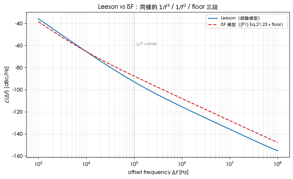
8. Simulation figure

9. How to read the figure

• Three-segment broken line: both curves, from left (close to carrier) to right (far offset), show $1/f^3$ (steepest) → $1/f^2$ (middle) → flat floor. The gray dotted line is the $1/f^3$ corner ($f_c=100$ kHz): to its left both curves are steeper ($-30$ dB/dec), to its right they turn to $-20$ dB/dec.
• Overlap in the middle, divergence at the ends: this lab deliberately tunes the parameters so the two curves nearly coincide in the $1/f^2$ region (teaching overlay). Note the right end (large offset) where the curves separate: Leeson's $(1+\ldots)$ factor has already flattened toward its constant floor, while the ISF model's floor is set lower at $-160$ dBc/Hz, so the red curve keeps following $1/f^2$ a while longer at high offset before hitting the floor. This difference is not a bug — the two models book the floor differently — a reminder that "the curve shape is right; absolute values depend on each model's parameters".
• Key reading: Leeson's $Q$ sets the mid-region corner, $F/P_s$ sets the floor; the ISF's $\Gamma_{rms}/q_{max}$ sets the mid-region height, $c_0$ sets the $1/f^3$ strength. One curve, two languages: to lower the middle region, lower $\Gamma_{rms}$ / raise $q_{max}$ (= raise $Q$, raise $P_s$); to lower close-in noise, suppress $c_0$ (= make the waveform symmetric).

10. Corresponding paper equations/figures

• ISF $1/f^2$ region: [P1] Eq.(21), p.185, $\mathcal{L}\propto\Gamma_{rms}^2/q_{max}^2/\Delta\omega^2$.
• ISF $1/f^3$ region: [P1] Eq.(23), p.185, $\propto c_0^2\cdot\omega_{1/f}/\Delta\omega^3$.
• $1/f^3$ corner (physical meaning, different from the device corner): [P1] Eq.(24), p.185.
• Full three-region picture: [P1] Fig. 11 / Fig. 12, p.185 ($1/f^3$, $1/f^2$, floor, and corner definitions).
• Leeson model: D. B. Leeson, Proc. IEEE, 1966, not among the five source PDFs, supplemented as external literature; step-by-step derivation and term-by-term comparison in derivation_leeson.

11. Limitations and approximations

• Leeson is an empirical model (external literature): $F$, $Q$, and the corner are mostly after-the-fact fits, unlike the ISF which derives them from circuit quantities ($\Gamma_{rms},q_{max},c_0$); the Leeson parameters in this figure are illustrative.
• Parameters deliberately co-tuned: the ISF-side $\Gamma_{rms}=0.5,c_0=0.2,$ floor$=-160$ dBc/Hz were chosen to make the curves coincide in the middle region, not extracted from any specific oscillator; do not read the absolute dBc/Hz as real device specs.
• Different floor bookkeeping: Leeson's floor is built into the $(1+\ldots)$ factor, while the ISF model uses an added constant floor; hence the divergence at high offset (see figure reading) — a model-structure difference, not a physical one.
• Single white source, linear region summation: the ISF model directly adds $1/f^2$ and $1/f^3$ in the linear power domain, ignoring multiple sources, cyclostationarity (see lab_14), and AM–PM.
• Factor-of-2: $1/f^2$ uses Eq.(21)'s $4\Delta\omega^2$, $1/f^3$ uses Eq.(23)'s $8\Delta\omega^2$; the minor factor-of-2 SSB-bookkeeping dispute does not affect the three-region slopes or the comparison conclusions.
• $Q=10$ is low: illustrative; real LC tanks often have $Q\gtrsim$ several tens, moving Leeson's mid-region corner closer to the carrier.

Key takeaways

• Free-running oscillator phase noise has three regions: $1/f^3$ (close-in) → $1/f^2$ (white noise) → flat floor.
• Leeson (empirical, external literature) and the ISF (derived in [P1]) describe the same three regions; the ISF gives Leeson's parameters physical meaning.
• $1/f^2$ height $=\Gamma_{rms}^2/q_{max}^2$ (↔ Leeson's $2FkT/P_s$ and $Q$); $1/f^3$ strength $=c_0^2$.
• The ISF's $1/f^3$ corner ([P1] Eq.(24)) scales with $c_0^2/\Gamma_{rms}^2$ and is not equal to the device $1/f$ corner.

Further reading

• White noise → $1/f^2$: lab_06_white_noise_phase_noise, white_noise_to_phase_noise
• Flicker upconversion → $1/f^3$ and $c_0$: lab_07_flicker_noise_upconversion, flicker_noise_upconversion
• Design trade-offs: lab_09_design_tradeoffs
• Applied to design/theory: step-by-step Leeson derivation and term-by-term "$Q,F,1/f^3$ corner" mapping onto the ISF → derivation_leeson