Lab 14 — Cyclostationary noise 與 effective ISF

麵包屑：模擬實驗室 › 系統與進階 › 本頁（cyclostationary／effective ISF）。上游：lab_06、effective_isf；相關：lab_09。

前面幾個 lab 都假設 noise 源「整個週期都一樣吵」（stationary，定常）。真實電路不是這樣： 一顆 tail current（尾電流源）或 switching transistor（切換電晶體）只在週期的某一段才導通、 才注入 noise。這種「noise 強度本身隨振盪相位週期性變化」的 noise 叫 cyclostationary noise（週期穩態雜訊）。這個 lab 用一個介於 0、1 之間的 noise-modulating function（NMF，雜訊調變函數） $\alpha(\theta)$ 把「device 何時吵」 畫出來，然後說明真正決定 phase noise 的不是原始 ISF，而是 effective ISF（有效 ISF） $\Gamma_{eff}=\Gamma\cdot\alpha$。

物理直覺（先講結論）：phase noise 不只看 device 多吵（$\overline{i_n^2}$），也看 它在波形的哪個相位吵。同一顆 device，若它最吵的時段剛好落在 ISF 很大的地方 （例如 zero crossing），它的破壞力就大；若落在 ISF≈0 的波峰，破壞力就小。把 「何時吵」$\alpha(\theta)$ 乘進 ISF，得到 $\Gamma_{eff}=\Gamma\alpha$，再對 $\Gamma_{eff}$ 取 rms，才是這顆 cyclostationary 源真正的有效敏感度 $\Gamma_{eff,rms}$。

1. 教學目標

• 理解 stationary（定常）與 cyclostationary（週期穩態）noise 的差別。
• 用 NMF $\alpha(\theta)\in[0,1]$ 模型化「device 只在週期的某段吵」。
• 推出 effective ISF $\Gamma_{eff}(\theta)=\Gamma(\theta)\,\alpha(\theta)$，並用它取代 $\Gamma$ 算 rms。
• 看懂：同一顆 device、同樣 noise 量，只因「注入相位」不同，$\Gamma_{eff,rms}$ 可以差好幾倍。

2. 數學模型

從 [P1] Eq.(21), p.185 的白噪 phase-noise 律出發：

$$\mathcal{L}\{\Delta\omega\}=10\log_{10}\!\left(\frac{\Gamma_{rms}^2}{q_{max}^2}\cdot\frac{\overline{i_n^2}/\Delta f}{4\,\Delta\omega^2}\right)$$

這條假設 $\overline{i_n^2}/\Delta f$ 是常數（stationary）。若 noise 是 cyclostationary， 其瞬時 PSD 可寫成「定常分量乘上一個週期 gate」：

$$\overline{i_n^2(\theta)}/\Delta f=\big(\overline{i_n^2}/\Delta f\big)\cdot\alpha^2(\theta),\qquad \alpha(\theta)\in[0,1].$$

把這個相位相依塞回 [P1] Eq.(11), p.182 的 ISF 積分核 $\Gamma(\omega_0\tau)\,i_n(\tau)$， 等效於把 noise 的「$\alpha$」併進 ISF。定義 effective ISF（規範第 10 節）：

$$\Gamma_{eff}(\theta)=\Gamma(\theta)\,\alpha(\theta).$$

於是 cyclostationary 源的 phase noise 就用 $\Gamma_{eff,rms}$ 取代 $\Gamma_{rms}$：

$$\Gamma_{eff,rms}=\sqrt{\frac{1}{2\pi}\int_0^{2\pi}\big[\Gamma(\theta)\,\alpha(\theta)\big]^2\,d\theta},$$

並用它代入 [P1] Eq.(21)：$\mathcal{L}\propto\Gamma_{eff,rms}^2/q_{max}^2$。

• 為何乘法是對的：$\alpha$ 描述「noise 振幅相對被 gate 的比例」，ISF 描述「該相位的 noise 轉成相位的效率」。兩者都作用在「同一時刻的注入」上，效果相乘。
• Dimension check：$\Gamma$ 無因次、$\alpha$ 無因次（$\in[0,1]$）⇒ $\Gamma_{eff}$ 無因次 ✓， 和原 ISF 同單位，可直接代進 Eq.(21)。

本 lab 用理想 LC 的 $\Gamma(\theta)=-\sin\theta$（[P1] 推導，最大 $\vert\Gamma\vert$ 在 zero crossing $\theta=\pi/2$、$\Gamma\approx0$ 在波峰 $\theta=0$），配兩個寬度同為 $\pi$ 的 平滑 gate：一個 gate 在 zero crossing（壞），一個在波峰（好）。

3. Block diagram

4. Python 核心 code

下面是 simulations/lab_14_cyclostationary_isf.py 的核心：用 gamma_lc_ideal（$-\sin$） 當 ISF，用平滑週期窗 nmf_window 當 $\alpha(\theta)$，再用 effective_isf（即 $\Gamma\cdot\alpha$） 與 gamma_rms 算各自的 rms。

import numpy as np
from simulations.common.isf_utils import gamma_lc_ideal, gamma_rms, effective_isf


def nmf_window(theta, center, width):
    """Smooth periodic gate in [0,1], centered at `center`, of given width (rad)."""
    d = np.angle(np.exp(1j * (theta - center)))  # wrapped distance
    return 0.5 * (1 + np.cos(np.pi * np.clip(d / (width / 2), -1, 1)))


theta = np.linspace(0, 2 * np.pi, 2000, endpoint=True)
gamma = gamma_lc_ideal(theta)                 # -sin(theta)

# case 1: device noisy near the ZERO CROSSING (where |Gamma| is max) -> bad
a_bad = nmf_window(theta, center=np.pi / 2, width=np.pi)
# case 2: device noisy near the PEAK (where |Gamma|~0) -> good
a_good = nmf_window(theta, center=0.0, width=np.pi)

g_bad = effective_isf(gamma, a_bad)           # Gamma * alpha
g_good = effective_isf(gamma, a_good)

grms = gamma_rms(theta, gamma)                # stationary reference
grms_bad = gamma_rms(theta, g_bad)
grms_good = gamma_rms(theta, g_good)
print(f"stationary={grms:.3f} bad={grms_bad:.3f} good={grms_good:.3f}")
# -> stationary=0.707, bad=0.395, good=0.177

effective_isf(gamma_values, alpha_values) 就是逐點相乘（見 simulations/common/isf_utils.py）， gamma_rms(theta, gamma) 是 $\sqrt{\frac{1}{2\pi}\int_0^{2\pi}\Gamma^2\,d\theta}$，對應 [P1] Eq.(20)。

5. 完整 script path

simulations/lab_14_cyclostationary_isf.py（main() 產生圖；NMF 用 nmf_window， effective ISF 與 rms 用 simulations/common/isf_utils.py 的 effective_isf、gamma_rms、 gamma_lc_ideal）。重跑：python scripts/run_all_sims.py。

6. 參數表

參數	符號	值	角色
ISF（理想 LC）	$\Gamma(\theta)$	$-\sin\theta$	固定（physically derived）
相位取樣點數	—	2000	一個週期 $[0,2\pi]$（含端點）
壞 gate 中心	$\theta_{c,\text{bad}}$	$\pi/2$	noise 落在 zero crossing（$\vert\Gamma\vert$ 最大）
好 gate 中心	$\theta_{c,\text{good}}$	$0$	noise 落在波峰（$\Gamma\approx0$）
gate 寬度	width	$\pi$	兩 case 相同（半個週期）
NMF 上下界	$\alpha$	$[0,1]$	平滑 raised-cosine 窗

7. 單位表

量	符號	單位
振盪相位	$\theta=\omega_0\tau$	rad
ISF	$\Gamma$	無因次
NMF	$\alpha$	無因次（$\in[0,1]$）
effective ISF	$\Gamma_{eff}=\Gamma\alpha$	無因次
rms ISF	$\Gamma_{rms},\Gamma_{eff,rms}$	無因次

8. 模擬圖

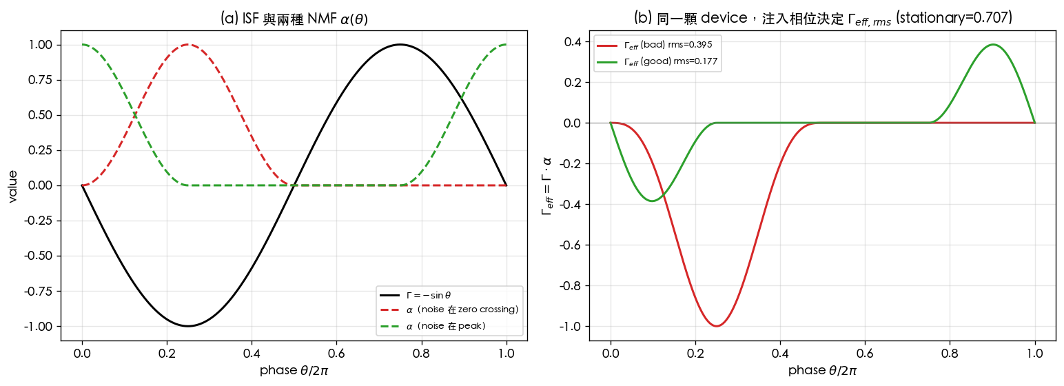
9. 如何解讀圖

• 左圖 (a)：黑線是 ISF $\Gamma=-\sin\theta$（在 $\theta/2\pi=0.25$、$0.75$ 即 zero crossing 處 $\vert\Gamma\vert$ 最大；在 $0$、$0.5$ 即波峰處 $\Gamma=0$）。紅虛線 $\alpha$ 把 device 的吵 時段放在 zero crossing（$\theta/2\pi\approx0.25$）；綠虛線 $\alpha$ 放在波峰（$\theta/2\pi\approx0$）。 兩個 gate 形狀、寬度完全一樣，只差相位。
• 右圖 (b)：把左圖相乘得 $\Gamma_{eff}=\Gamma\alpha$。紅線（壞）在 zero crossing 撞上 ISF 的 大值，留下一個又深又寬的 lobe，$\Gamma_{eff,rms}=0.395$；綠線（好）落在波峰，ISF 幾乎為 0， 只剩兩側殘餘小 lobe，$\Gamma_{eff,rms}=0.177$。
• 關鍵讀法：stationary 參考 $\Gamma_{rms}=0.707$（=$1/\sqrt2$，$-\sin$ 整週的 rms）。 一旦 gate 只開半週，rms 一定下降；但下降多少完全看 gate 對到 ISF 的哪裡：壞 case 仍有 $0.395$，好 case 砍到 $0.177$，差約 $2.2$ 倍。 phase noise 差 $20\log_{10}(0.395/0.177)\approx7$ dB。同一顆 device、同樣 noise 量，只改注入相位就賺 7 dB。

10. 對應 paper 公式/figure

• 白噪 phase noise（用 $\Gamma_{eff,rms}$ 取代 $\Gamma_{rms}$）：[P1] Eq.(21), p.185。
• ISF 積分核（$\Gamma\cdot i_n$，$\alpha$ 併入處）：[P1] Eq.(11), p.182。
• Parseval / rms：[P1] Eq.(20), p.185，$\sum_n c_n^2=2\Gamma_{rms}^2$。
• cyclostationary noise 概念：[P1] Sec. II-D「Cyclostationary Noise Sources」， Eq.(25)–(27), p.186。其中 $i_n(t)=i_{n0}(t)\,\alpha(\omega_0 t)$ 為 Eq.(25)、代回積分為 Eq.(26)， 而 effective ISF $\Gamma_{eff}(x)=\Gamma(x)\cdot\alpha(x)$ 即 Eq.(27)；本 lab 是其 toy 視覺化。
• 概念延伸：device 的 $\alpha$ 從哪來、如何 mapping，見 device_noise_mapping 與 effective_isf。

11. 限制與 approximation

• toy model，非 transistor-level：$\alpha(\theta)$ 用人工 raised-cosine 窗，不是從電晶體 $g_m$／導通區間萃取的真實 NMF；ISF 用理想 LC 的 $-\sin$。真實 device 的 $\alpha$ 與 $\Gamma$ 都要靠 PSS／transient 模擬萃取。
• $\Gamma_{eff}=\Gamma\alpha$ 是一階近似：假設 noise 振幅被 gate 線性調變、且 $\alpha$ 與相位 響應相互獨立；忽略 noise 自身的 AM–PM 與 $\alpha$、$\Gamma$ 間的耦合。
• 只示意 rms，未跑 PSD：本 lab 用 $\Gamma_{eff,rms}$ 說明 scaling，沒有把 cyclostationary 源實際丟進 [P1] Eq.(11) 積分跑出 PSD（那會是 lab_06 的延伸）。
• 單一源：真實電路多個 cyclostationary 源各有自己的 $\alpha$，要分別算 $\Gamma_{eff,rms}$ 再對功率求和。
• factor-of-2：沿用 Eq.(21) 的 $4\Delta\omega^2$ 慣例；SSB 記帳的 2 倍差異不影響此處所有 相對（dB）比較。

重點回顧

• cyclostationary noise：noise 強度隨振盪相位週期變化，用 $\alpha(\theta)\in[0,1]$ 描述。
• effective ISF：$\Gamma_{eff}=\Gamma\cdot\alpha$；phase noise 用 $\Gamma_{eff,rms}$ 取代 $\Gamma_{rms}$ 代入 [P1] Eq.(21)。
• 本 lab 數字：stationary $\Gamma_{rms}=0.707$；noise 在 zero crossing → $0.395$（壞）；在波峰 → $0.177$（好）。
• 設計含義：把吵的 device 安排在 ISF 小的相位（波峰）注入，可省可觀 phase noise。

延伸閱讀

• effective ISF 理論：effective_isf
• 白噪 → phase noise（stationary 版）：lab_06_white_noise_phase_noise
• 設計取捨總整理：lab_09_design_tradeoffs
• 用在設計/理論：device 的 $\alpha(\theta)$ 從 bias/導通區間怎麼 mapping 出來 → device_noise_mapping