β: This English translation is in beta — the Traditional-Chinese original is the authoritative version.

Lab 04 — impulse injection sweep and LTI vs LTV

This lab turns the "operational ISF definition" from impulse_to_phase_shift into a measurable experiment: inject a very small charge impulse at different phases $\theta=\omega_0\tau$ of the waveform, measure the permanent phase shift it causes, divide that shift by the injected amount, and thereby back out the ISF (impulse sensitivity function — where on its waveform the oscillator is most vulnerable to a kick).

The extracted numerical ISF nearly coincides with the analytic solution $\Gamma(\theta)=-\sin\theta$ for the ideal LC (maximum error about $7\times10^{-4}$). The same lab also uses impulse responses to draw out the difference between LTI (linear time-invariant) vs LTV (linear time-variant — the system parameters vary periodically with time) — the key reason the whole ISF theory "cannot treat oscillator phase with an ordinary LTI transfer function."

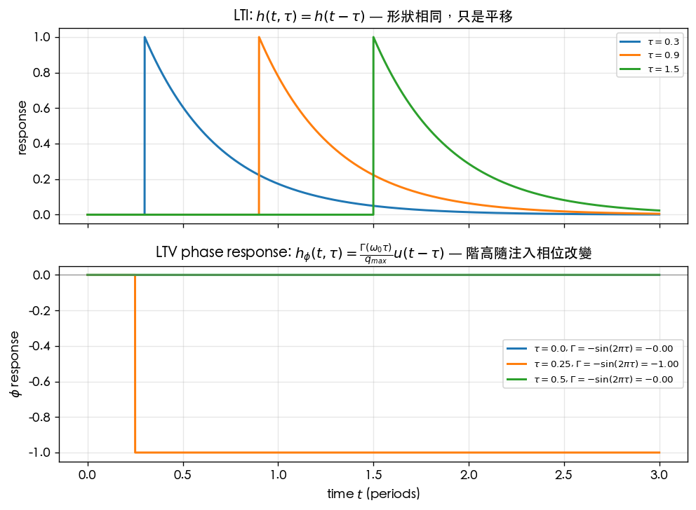
The two things this lab wants you to see with your own eyes: (1) the ISF is not an abstract definition; it is the result of the action "kick at phase $\theta$, measure the persistent phase jump"; (2) the same-size impulse barely changes the phase when it kicks at the peak, but causes the largest phase jump at the zero crossing — this "kick effect varying periodically with the injection instant" is LTV, and can never be drawn by an LTI impulse response that depends only on $t-\tau$.

1. Learning objectives

• Turn the operational ISF definition $\Delta\phi=\dfrac{\Gamma(\omega_0\tau)}{q_{max}}\,\Delta q$ into a numerical experimental flow: sweep the injection phase → measure the persistent phase → back out $\Gamma$.
• Verify that the ISF of the ideal LC oscillator (current injected into the capacitor node) is exactly $\Gamma(\theta)=-\sin\theta$, and quantify the numerical-vs-theory error (~$10^{-3}$ level).
• Understand the difference between the "persistent phase shift" and the "decaying amplitude perturbation" — only the tangential (phase) component remains permanently.
• Use the impulse-response comparison plot to build the physical picture of LTV: the step height varies periodically with the injection phase.
• Maps to [P1] Eq.(10),(11) and Fig. 4.

2. Mathematical model

The whole lab stands on this LTV impulse response ([P1] Eq.(10), p.182):

$$h_\phi(t,\tau)=\frac{\Gamma(\omega_0\tau)}{q_{max}}\,u(t-\tau)$$

Its meaning: injecting unit charge at time $\tau$ (corresponding to phase $\omega_0\tau$) makes the phase jump in a single step to $\Gamma(\omega_0\tau)/q_{max}$, and because of the unit step $u(t-\tau)$ the jump is kept permanently. Superposing it over all past noise currents gives the central LTV phase response ([P1] Eq.(11), p.182):

$$\phi(t)=\frac{1}{q_{max}}\int_{-\infty}^{t}\Gamma(\omega_0\tau)\,i_n(\tau)\,d\tau$$

The single-impulse experiment that backs out the ISF: if $i_n$ is just one narrow pulse located at phase $\theta$ with total charge $\Delta q$, Eq.(11) degenerates to a single step (the step version of [P1] Eq.(10); see also the operational definition in impulse_to_phase_shift):

$$\Delta\phi(\theta)=\frac{\Gamma(\theta)}{q_{max}}\,\Delta q \quad\Longrightarrow\quad \Gamma(\theta)=\frac{\Delta\phi(\theta)}{\Delta q/q_{max}} .$$

• dimension check: the right-hand side $[\text{rad}]/(\text{C}/\text{C})=[\text{rad}]$ looks like it carries units, but $\Delta\phi$ is rad (dimensionless) and $\Delta q/q_{max}$ is dimensionless, so $\Gamma$ is dimensionless ✓.
• Theory reference: for the ideal lossless parallel LC with current injected into the capacitor node, the state is $z=(v,w)=A(\cos\theta,\sin\theta)$; a charge impulse pushes $v$ by $\Delta v=\Delta q/C$, and projecting onto the limit-cycle tangential direction gives $\Delta\phi=-(\sin\theta)\,\Delta v/A$; combined with $q_{max}=CA$ this yields

$$\boxed{\ \Gamma(\theta)=-\sin\theta\ }$$

At the peak $\theta=0$, $\Gamma=0$ (pure amplitude change); at the zero crossing $\theta=\pi/2$, $|\Gamma|$ is maximum (pure phase change). Full geometric derivation: isf_definition.

The mathematical difference of LTV vs LTV: an LTI system's impulse response depends only on the time difference, $h(t,\tau)=h(t-\tau)$; the oscillator's phase impulse response $h_\phi(t,\tau)$ explicitly depends on the absolute injection instant $\tau$ (through the $2\pi$-periodic weight $\Gamma(\omega_0\tau)$) — precisely the definition of LTV.

3. Block diagram

4. Core Python code

The core of backing out the ISF is extract_isf_by_injection: for each phase $\theta$ run one injection simulation, measure the mean phase difference over "the last period" relative to a no-injection reference trajectory (this keeps only the permanent phase and filters out the already-decayed amplitude perturbation), then divide by $\Delta q/q_{max}$. Quoted verbatim from the real code (simulations/common/oscillator_models.py):

def extract_isf_by_injection(f0, fs, n_inject_periods=6, settle_periods=4,
                             dq_over_qmax=1e-3, n_points=64, mu=0.3):
    T = 1.0 / f0
    settle = settle_periods * T
    t_end = (settle_periods + n_inject_periods) * T
    thetas = np.linspace(0.0, TWO_PI, n_points, endpoint=False)
    gamma_num = np.zeros(n_points)

    # Reference (no impulse), started from the limit cycle.
    t_ref, xr, yr = simulate_lc(f0, t_end, fs, mu=mu, x0=1.0, y0=0.0)
    phi_ref = excess_phase(t_ref, xr, yr, f0)

    for i, th in enumerate(thetas):
        t_inj = settle + th / (TWO_PI * f0)  # phase th occurs at this time
        t_p, xp, yp = simulate_lc(f0, t_end, fs, mu=mu, x0=1.0, y0=0.0,
                                  impulse_time=t_inj, impulse_dx=dq_over_qmax)
        phi_p = excess_phase(t_p, xp, yp, f0)
        # persistent phase difference measured over the last period
        m = t_p >= (t_end - T)
        dphi = np.mean(phi_p[m] - phi_ref[m])
        gamma_num[i] = dphi / dq_over_qmax

    gamma_analytic = -np.sin(thetas)
    return thetas, gamma_num, gamma_analytic

The core of the LTV vs LTV comparison figure plots "LTI: step height fixed, only time-shifted" next to "LTV: step height $=\Gamma(\omega_0\tau)$ varying with the injection phase" (simulations/lab_04_impulse_sweep.py):

    # LTV (oscillator phase): step of height Gamma(w0 tau)/qmax * u(t - tau).
    ax = axes[1]
    for tau, c in zip([0.0, 0.25, 0.5], ["tab:blue", "tab:orange", "tab:green"]):
        gamma = -np.sin(2 * np.pi * f0 * tau)  # ISF at injection phase
        h = gamma * (t >= tau)
        ax.plot(t, h, color=c,
                label=fr"$\tau={tau}$, $\Gamma=-\sin(2\pi\tau)={gamma:+.2f}$")

• Why measure "the mean over the last period": the transient right after injection contains both an amplitude perturbation and a phase jump; the Van der Pol-type amplitude restoration with mu=0.3 pulls the radial (amplitude) component back to the limit cycle within a few periods, leaving only the tangential (phase) component permanently. Measuring after n_inject_periods periods yields the clean persistent phase.
• Why endpoint=False: $\theta=0$ and $\theta=2\pi$ are the same phase — do not duplicate it in the sweep.
• Why dq_over_qmax=1e-3 is small: keeps small-signal linearity ($\Delta q\ll q_{max}$); otherwise the ISF itself would be altered by the large injection and the extraction would be inaccurate.

5. Full script path

simulations/lab_04_impulse_sweep.py (calls simulate_lc, excess_phase, extract_isf_by_injection from simulations/common/oscillator_models.py; plotting utilities in simulations/common/plot_utils.py). How to run: python scripts/run_all_sims.py; figures are written to static/figures/.

6. Parameter table

Parameter	Code variable	Value	Notes
Oscillation frequency	f0	1.0 (normalized)	the toy model uses a dimensionless frequency; the real-world 5 GHz mapping is in the units table below
Sampling rate	fs	8000 (sweep) / 2000 (LTV figure)	$fs/f_0$ points per period, enough to resolve the tangential projection
Injected charge ratio	dq_over_qmax	$10^{-3}$	$\Delta q/q_{max}$, keeps small signal
Sweep points	n_points	48	48 injection phases within one period
Post-injection observation	n_inject_periods	6	run 6 more periods after injection so the amplitude perturbation decays
Settle periods	settle_periods	4	let the system settle onto the limit cycle before injecting
Restoration strength	mu	0.3	Van der Pol-type amplitude restoration; $\mu=0$ is the ideal lossless LC
LTV-figure injection phases	tau	0.0, 0.25, 0.5 (periods)	correspond to $\Gamma=-\sin(2\pi\tau)=0,-1,0$

7. Units table

Quantity	Symbol	toy-model unit	Physical unit
Time	$t,\tau$	periods (normalized)	s
Injection phase	$\theta=\omega_0\tau$	rad ($2\pi$-periodic)	rad
Injected charge ratio	$\Delta q/q_{max}$	dimensionless	C/C
Persistent phase	$\Delta\phi$	rad	rad
ISF	$\Gamma(\theta)$	dimensionless	—
Maximum error	$\max\vert \Gamma_{num}-\Gamma_{ana}\vert$	dimensionless	—

toy model note: this is a pedagogical toy model (2-D Van der Pol-type state-space), not transistor-level. It faithfully reproduces the mechanism of the ISF (tangential projection, $-\sin\theta$, LTV) but does not produce real-circuit numbers. To convert into physical intuition, apply canonical example A: $q_{max}=1$ pC, $\Delta q=1$ fC (i.e. $\Delta q/q_{max}=10^{-3}$), $\Gamma=0.5$, $f_0=5$ GHz $\Rightarrow$ $\Delta\phi=5\times10^{-4}$ rad, $\Delta t=15.9$ fs.

8. Simulation figures

Figure 1: phase shift vs injection phase — the same $\Delta q/q_{max}=10^{-3}$ impulse, kicked at different phases, produces completely different persistent $\Delta\phi$:

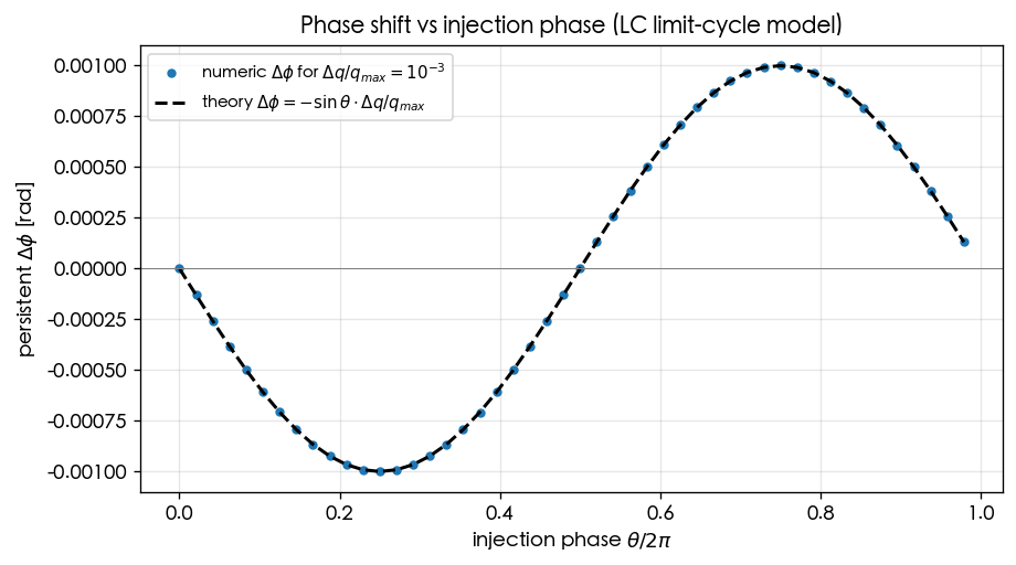
Figure 2: numerically extracted ISF vs theoretical −sinθ — dividing the vertical axis of the previous figure by $\Delta q/q_{max}$ gives the ISF itself; the numerical points (purple circles) nearly coincide with the theoretical dashed line:

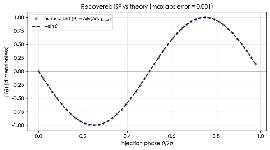
Figure 3: LTI vs LTV impulse responses — top: the LTI response keeps its shape and only shifts; bottom: the LTV step height varies with the injection phase:

9. How to read the figures

Figure 1 (phase sweep): the horizontal axis is the injection phase $\theta/2\pi$ (one period), the vertical axis is the persistent phase shift $\Delta\phi$. Note that it is a $-\sin$-shaped curve: nearly zero at $\theta=0$ (the peak), the largest negative value at $\theta\approx0.25$ (rising zero crossing), the largest positive value at $\theta\approx0.75$. This is direct evidence of LTV — the effect of "the same kick" depends entirely on "where on the waveform you kick." The numerical blue circles hug the black theoretical dashed line.

Figure 2 (recovered ISF): dividing Figure 1 by $\Delta q/q_{max}=10^{-3}$ gives $\Gamma(\theta)$. The title reports a maximum absolute error of about $7\times10^{-4}$ (the title is formatted to three decimals, about 0.001). Error sources: RK4 time discretization, the $\theta$ sampling (48 points), and the measurement window averaging only over the last period. This level is enough to claim "the numerical method successfully recovered $\Gamma=-\sin\theta$ of the ideal LC."

Figure 3 (LTI vs LTV):

• Top half (LTI): the three curves are the same decaying-exponential impulse response shifted to $\tau=0.3,0.9,1.5$ — identical shape, only the starting point differs. This is the LTI hallmark: $h(t,\tau)=h(t-\tau)$.
• Bottom half (LTV phase): all three are unit steps (permanently held), but with different step heights: at $\tau=0$, $\Gamma=-\sin(0)=0$ (kick at the peak, phase unmoved); at $\tau=0.25$, $\Gamma=-\sin(\pi/2)=-1$ (kick at the zero crossing, largest phase jump); at $\tau=0.5$, $\Gamma=-\sin(\pi)=0$. The step height varies with the absolute injection phase — this is LTV, and the fundamental reason a single LTI transfer function cannot describe oscillator phase.

10. Corresponding paper equations / figures

• [P1] Eq.(10), p.182: $h_\phi(t,\tau)=\dfrac{\Gamma(\omega_0\tau)}{q_{max}}\,u(t-\tau)$ — every curve in the bottom half of Figure 3 is exactly this (a different $\tau$ gives a different step height $\Gamma(\omega_0\tau)$).
• [P1] Eq.(11), p.182: $\phi(t)=\dfrac{1}{q_{max}}\displaystyle\int_{-\infty}^{t}\Gamma(\omega_0\tau)\,i_n(\tau)\,d\tau$ — this lab is its single-impulse special case (the basis for backing out $\Gamma$).
• [P1] Fig. 4, p.181: caption "(a) impulse injected at the peak, (b) impulse injected at the zero crossing, and (c) effect of nonlinearity on amplitude and phase ... in state-space" — demonstrates the difference between impulses injected at the peak vs the zero crossing, and the effect of nonlinearity on amplitude/phase (state-space picture). Figures 1/2 of this lab are its toy-model reproduction on the ideal LC (TODO: only the exact axis-tick values of Fig. 4 have not yet been transcribed verbatim; check the original figure on [P1] p.181).
• Geometric derivation of the $-\sin\theta$ ISF: see isf_definition; operational definition and the 16 fs numerical example: impulse_to_phase_shift.

11. Limitations and approximations

Limitation / approximation	Impact	Where it holds / fails
2-D Van der Pol toy model (not transistor-level)	Reproduces the mechanism only, gives no real-circuit numbers	Sufficient for teaching; for design, extract $\Gamma$ with transient/adjoint
Small signal $\Delta q/q_{max}=10^{-3}$	$\Delta\phi$ linearly proportional to $\Delta q$	Large injection → nonlinearity, AM–PM, $\Gamma$ itself altered
Measure only after mu=0.3 has let the amplitude perturbation decay	Needed to isolate the pure phase component	If $\mu$ is too small and the amplitude perturbation has not fully decayed, the measured $\Delta\phi$ is contaminated by residual amplitude
RK4 + finite fs discretization	Introduces ~$10^{-3}$ numerical error	Raising fs/n_points lowers it further, but this lab's level is already sufficient
Ideal lossless LC's $\Gamma=-\sin\theta$	Holds only for injection into the single capacitor node	Multi-node, ring, and lossy cases have different ISF shapes (see lab_05 and the ring model)
The LTI reference curve is an illustrative exponential decay	Only to contrast "shape invariance"	It is not the impulse response of any real circuit — purely a teaching reference

Key takeaways

• The ISF is measurable: inject a small charge at phase $\theta$, measure the persistent $\Delta\phi$, divide by $\Delta q/q_{max}$.
• The ISF backed out of the ideal LC (capacitor-node injection) is exactly $\Gamma(\theta)=-\sin\theta$; maximum numerical-vs-theory error ~$10^{-3}$.
• Injection at the peak → pure amplitude change (pulled back); injection at the zero crossing → pure phase change (permanently retained).
• The essence of LTV: the phase impulse response $h_\phi(t,\tau)$ depends on the absolute injection phase, with step height $=\Gamma(\omega_0\tau)$ — not on $t-\tau$ alone.
• Source: [P1] Eqs.(10),(11), p.182 and Fig. 4.

Further reading

• Operational definition and physical intuition: impulse_to_phase_shift
• Geometric derivation of $-\sin\theta$: isf_definition
• Decomposing the ISF into Fourier coefficients: lab_05
• Numerical conversion feel: numerical_feeling