From Impulse to Phase Shift — the Derivation

β: This English translation is in beta — the Traditional-Chinese original is the authoritative version.

Prerequisites: oscillator_phase (limit-cycle and phase/amplitude geometry), lti_vs_ltv (why an oscillator is LTV with respect to noise) | Up next: isf_definition (the rigorous ISF definition and the multi-node picture) → convolution_derivation (superposing arbitrary noise by convolution)

This page answers a very concrete question: when a current impulse is injected into some node of an oscillator, by how much does the oscillator's phase shift? The answer is the operational definition at the heart of ISF theory:

$$\Delta\phi=\frac{\Gamma(\omega_0\tau)}{q_{max}}\,\Delta q$$

We will not simply memorize this line — we will derive it from the capacitor relation $q=Cv$, one step at a time, stating at every step which physics is invoked, which approximation is made, what the units are, and how to run the dimension check.

Physical intuition (conclusion first): the noise current first becomes a packet of charge $\Delta q$ on the node; that charge nudges the oscillator's instantaneous state slightly off its steady orbit; how much of that nudge turns into phase and how much into amplitude depends on at which phase of the waveform you deliver the kick — and that conversion ratio is precisely the ISF $\Gamma$. Kick where the waveform slope is large and the phase gets pushed a lot; kick at the peak and you mostly perturb the amplitude.

Step 1: the current impulse becomes charge

Current integrated over time is charge. A very narrow, very short current pulse $i(t)$ injected into the node deposits a total charge

$$\Delta q=\int i(t)\,dt .$$

• Physics used: charge conservation / the definition of current, $i=dq/dt$.
• Unit check: $[\text{A}]\cdot[\text{s}]=[\text{C}]$ ✓ (amperes times seconds are coulombs).
• Why this is legitimate: when the pulse width is far smaller than the period $T$, the injection can be treated as dumping $\Delta q$ onto the node "instantaneously".

Step 2: charge becomes a voltage step

The node carries a total capacitance $C_{node}$. Charge appearing instantaneously makes the node voltage jump by a step ([P1] Eq.(9), p.181):

$$\Delta V=\frac{\Delta q}{C_{node}} .$$

• Physics used: the capacitor relation $q=Cv$; differentiate for a small change, $\Delta q=C\,\Delta V$.
• Unit check: $[\text{C}]/[\text{F}]=[\text{C}]/[\text{C/V}]=[\text{V}]$ ✓.
• Key observation: in a parallel LC, a current impulse changes only the capacitor voltage (instantaneously); it cannot change the inductor current (an inductor current cannot jump). In state space, the perturbation is therefore a horizontal displacement along the voltage axis.

Step 3: the voltage step pushes the state off the limit cycle — but only the tangential component becomes phase

Draw the oscillator's state in a 2-D plane (say, horizontal axis = capacitor voltage $v$, vertical axis = $w$, proportional to the inductor current). In steady state, the state point circulates along the limit cycle. The voltage jump from Step 2 shoves the state point sideways:

• The radial component, pushing away from the cycle → changes the amplitude $A$. But the oscillator has an amplitude-restoring mechanism, so this part is slowly pulled back and leaves no permanent residue.
• The tangential component, along the cycle → changes the phase $\phi$. Phase has no restoring force, so this part stays forever.

The same $\Delta V$, kicked at a different phase $\tau$, splits differently between tangential and radial. Collect the "$\Delta V$-to-$\Delta\phi$ conversion ratio" into a periodic function that depends only on the injection phase — that is the ISF:

$$\Delta\phi=\underbrace{\big(\text{phase-conversion ratio}\big)}_{\text{depends only on }\omega_0\tau}\times\Delta V .$$

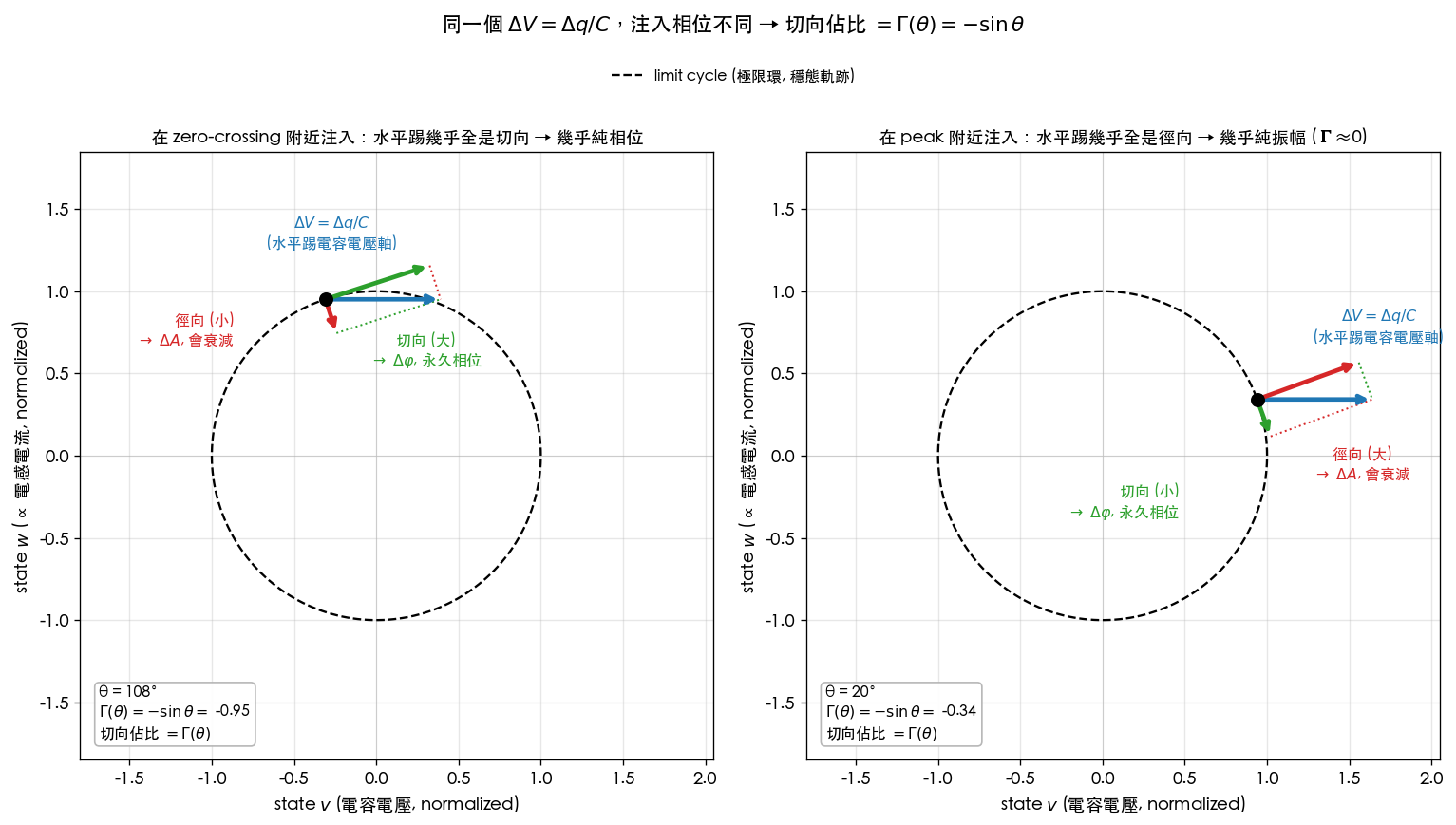
The figure below draws this decomposition on the state plane. The same packet of charge produces a horizontal $\Delta V=\Delta q/C$ (the current kicks only the capacitor-voltage axis; the inductor current cannot jump), which the dashed lines split into a tangential component along the cycle (green — permanent phase) and a radial component off the cycle (red — decays). Injected near the zero crossing, the horizontal kick lands almost entirely on the tangent (the phase gets pushed a lot); injected near the peak, it lands almost entirely on the radius (only the amplitude changes). The lower-left corner of each panel prints the value of $\Gamma(\theta)=-\sin\theta$ — the tangential fraction is exactly $\Gamma(\theta)$, which makes the ideal-LC $\Gamma=-\sin\theta$ geometrically inevitable (the algebraic derivation of $\Gamma=-\sin\theta$ is in isf_definition).

• Math used: project the perturbation vector onto the tangent direction (the phase direction) of the limit cycle.
• Why only the tangential part is kept: see phase_vs_amplitude_noise and oscillator_phase — amplitude is pulled back by the restoring mechanism; phase is not.

Step 4: normalize by $q_{max}$ to get the dimensionless ISF

Chain Steps 1–3 together: $\Delta\phi\propto\Delta V=\Delta q/C_{node}$. Hajimiri–Lee chose to normalize by the node's maximum charge swing $q_{max}=C_{node}V_{max}$, writing that "phase-conversion ratio" as the dimensionless function $\Gamma(\omega_0\tau)$ ([P1] Eq.(10)–(11), p.182):

$$\boxed{\ \Delta\phi=\frac{\Gamma(\omega_0\tau)}{q_{max}}\,\Delta q\ }$$

• Why the $q_{max}$ normalization: it turns $\Gamma$ into a dimensionless, amplitude-independent "shape" that describes only where the waveform is sensitive. The actual magnitude of the phase shift is set by $\Delta q/q_{max}$ (the injected charge relative to the signal charge).
• Why $\Gamma$ is dimensionless: $\Delta\phi$ is in rad (dimensionless) and $\Delta q/q_{max}$ is dimensionless, so $\Gamma$ must be dimensionless. Dimension check: $[\text{rad}]=\Gamma\cdot[\text{C}]/[\text{C}]$ $\Rightarrow\Gamma$ dimensionless ✓.
• Small-signal assumption: Step 3 treats the projection as linear, which requires $\Delta q\ll q_{max}$ (the kick must not knock the oscillator over). [P1] Fig. 6 confirms, on an actual Colpitts and a 5-stage ring, that $\Delta\phi$ is proportional to $\Delta q$ for small charge.

The corresponding impulse response (setting up the next chapter)

Because the phase step is retained forever, writing it as an impulse response brings along a unit step $u(t-\tau)$ ([P1] Eq.(10)):

$$h_\phi(t,\tau)=\frac{\Gamma(\omega_0\tau)}{q_{max}}\,u(t-\tau).$$

Note that it depends on the absolute injection instant $\tau$ (through $\Gamma(\omega_0\tau)$), not merely on $t-\tau$ — the very signature of an LTV (linear time-variant) system. The next chapter, convolution_derivation, uses it to superpose an arbitrary noise current. The complete ISF definition and the multi-node discussion are in isf_definition.

Numerical example (building a feel for the numbers)

Example A: $q_{max}=1$ pC, $\Delta q=1$ fC, $\Gamma=0.5$, $f_0=5$ GHz.

Phase step:

$$\Delta\phi=\frac{\Gamma\,\Delta q}{q_{max}}=\frac{0.5\times(1\times10^{-15}\,\text{C})}{1\times10^{-12}\,\text{C}}=5\times10^{-4}\ \text{rad}.$$

In degrees: $\Delta\phi=5\times10^{-4}\times\dfrac{180}{\pi}\approx0.0286^\circ$.

Converted to a timing error (using $\Delta t=\Delta\phi/(2\pi f_0)$):

$$\Delta t=\frac{5\times10^{-4}\ \text{rad}}{2\pi\times5\times10^{9}\ \text{Hz}}=\frac{5\times10^{-4}}{3.1416\times10^{10}}\ \text{s}\approx1.59\times10^{-14}\ \text{s}=15.9\ \text{fs}.$$

• Dimension check: $[\text{rad}]/[\text{rad/s}]=[\text{s}]$ ✓ (note that $2\pi f_0$ carries units of rad/s).
• Feel for the numbers: at 5 GHz (a 200 ps period), a single 1 fC packet of charge (about 6240 electrons) causes only ~16 fs of timing error even at the most sensitive phase. One kick is tiny — but the noise kicks continuously, and the integral accumulates (next chapter).

Quick verification with the built-in functions:

from simulations.common.isf_utils import impulse_to_phase_step
from simulations.common.noise_utils import phase_to_time_error

dphi = impulse_to_phase_step(delta_q=1e-15, gamma_value=0.5, qmax=1e-12)
dt   = phase_to_time_error(dphi, f0=5e9)
print(dphi, "rad", dt*1e15, "fs")   # -> 0.0005 rad  15.92 fs

(Full scripts: simulations/common/isf_utils.py, simulations/common/noise_utils.py.)

Seeing is believing: measuring $\Gamma$ directly

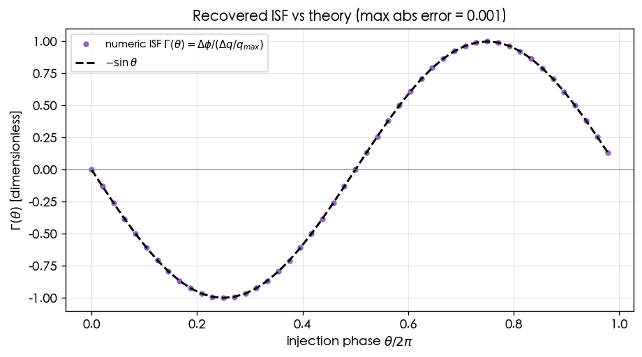
lab_04 injects a small charge at a sweep of phases in simulation, measures the persistent phase offset, and back-solves for the ISF; the result agrees almost perfectly with the ideal-LC $\Gamma(\theta)=-\sin\theta$ (maximum error about 0.001):

Where it applies, where it fails

Condition	When it holds	What happens when it fails
Small signal $\Delta q\ll q_{max}$	$\Delta\phi$ is linearly proportional to $\Delta q$	large injection → nonlinearity, AM–PM, and the ISF itself is altered
Amplitude perturbations decay	only the phase needs tracking	breaks down with strong AM–PM or without a stable limit cycle
Pulse far narrower than the period	can be treated as an instantaneous injection	wide pulses require the integral form, Eq.(11)
The correct $\Gamma$ is known	predictions are accurate	$\Gamma$ must be extracted by transient/adjoint simulation (see effective_isf)

Key takeaways

• Noise current → charge $\Delta q$ → voltage jump $\Delta V=\Delta q/C$ → projected through the ISF into phase $\Delta\phi$.
• $\Delta\phi=\Gamma(\omega_0\tau)\,\Delta q/q_{max}$; $\Gamma$ is dimensionless, $2\pi$-periodic, and depends on the injection phase.
• $q_{max}$ normalizes $\Gamma$ into a "shape"; the magnitude of the phase shift is set by $\Delta q/q_{max}$.
• A single 1 fC at 5 GHz, with $\Gamma=0.5$ and $q_{max}=1$ pC → 16 fs.
• Sources: [P1] Eq.(9) p.181, Eqs.(10),(11) p.182; verification figure in lab_04.

Further reading

• The geometry one step upstream: oscillator_phase
• The rigorous ISF definition and multiple nodes: isf_definition
• Superposing arbitrary noise: convolution_derivation
• Numerical feel, all in one place: numerical_feeling