β: This English translation is in beta — the Traditional-Chinese original is the authoritative version.

LC vs ring oscillator through the ISF lens

Prerequisites: tank_swing ($\mathcal{L}\propto\Gamma_{rms}^2/q_{max}^2$ and the swing lever), tank_Q_and_energy_restoration (what LC's "high-$Q$ energy storage" actually buys, why ring lacks this advantage), rms_isf ($\Gamma_{rms}$, Parseval, ring's $N^{-3/2}$ scaling) | Next: serdes_clocking_connection, varactor_tuning_supply_pushing

This page treats the ISF as a single unified ruler and measures the difference between LC and ring oscillators item by item. The point is not "which is better" (each has its use) but what the ISF framework lets us see, and what it doesn't. We first build an explicitly-labeled honest toy model, then quantify the differences using the [P1] / [P2] formulas.

Physical intuition (conclusion first): LC is like a heavy pendulum — most of the energy is stored in the tank ($L$ and $C$ trading back and forth), with only a small device occasionally topping up the loss. The waveform is close to sinusoidal, the ISF is smooth ($-\sin$), and phase sensitivity is spread across the whole period. ring is like a row of relay-passing gates — no energy-storage element, every stage is switching, every stage leaks noise, the waveform is close to a square wave, the ISF is concentrated at the transition, and phase sensitivity is sharp. LC buys low phase noise with "energy storage + high $Q$"; ring trades phase noise for "small area, tunability, multiphase output."

Toy model assumptions (explicitly labeled)

The following is a pedagogical toy model, not transistor-level. It captures the qualitative difference but is not a measurement of any real circuit.

• LC: ideal sinusoidal state, $V(\theta)=\cos\theta$, ISF $\Gamma_{LC}(\theta)=-\sin\theta$ ([P1] Fig. 7(a)). Amplitude restoration is provided by the limit cycle ([P1] Sec. III-A).
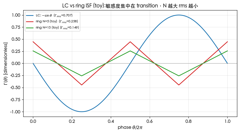
• ring: $N$-stage inverter delay + independent timing noise per stage; ISF modeled as a triangular toy shape, peak $\sim1/\sqrt{N}$, energy concentrated at the transition (actual simulated ISF curve: [P2] Fig. 5, p.793; triangular approximation: [P2] Fig. 6, p.793). Accumulated jitter uses a random-walk model $\sigma_{\Delta t}=\sigma_{edge}\sqrt{\Delta N}$ ([P2] Eq.(8)).
• Full scripts: simulations/lab_02_lc_toy_model.py, simulations/lab_03_ring_toy_model.py.

Item-by-item comparison table

Aspect	LC oscillator	Ring oscillator	How the ISF explains it
Waveform	Close to sinusoidal	Close to square (rail-to-rail)	Determines ISF shape (smooth vs. concentrated at transition)
ISF shape	$-\sin\theta$, smooth, spread over the full period	Triangular, sharp, concentrated at transition	See [P1] Fig. 7
Amplitude restoration	Tank + nonlinear $g_m$, radial perturbation decays	Each stage saturates to the rail, strong restoration	Amplitude perturbation decays → only phase is tracked (claim C2)
Transition slope	Moderate (sinusoidal zero-crossing slope)	Steep (fast switching)	Steep edge → low threshold jitter, concentrated $\Gamma_{rms}$
Stored energy (tank energy)	High ($L$, $C$ trade back and forth)	Almost none	High stored energy → large $q_{max}$ → low phase noise
Number of noisy devices	Few (1-2 active devices)	Many ($N$ stages, each leaks noise)	More noise sources contribute more (but each stage has smaller swing)
Phase-sensitivity distribution	Spread over the whole period	Concentrated in the transition window	$\Gamma_{eff}=\Gamma\cdot\alpha$ concentrated
$\Gamma_{rms}$	$0.5$ (rms of $-\sin$)	$\Gamma_{rms}\propto N^{-3/2}$ ([P2] Eq.16)	[P2] Eq.(16)
Jitter accumulation	Slow (high-$Q$ resists drift)	Fast (no reference, random walk)	$\sigma_{\Delta t}=\kappa\sqrt{\Delta t}$
Typical phase noise	Low (10-30 dB better)	High	$\propto\Gamma_{rms}^2/q_{max}^2$
Area / tunability / multiphase	Large (spiral inductor), narrow tuning range	Small, wide tuning, inherently multiphase output	(not an ISF quantity, but a common design metric)

Step 1: $\Gamma_{rms}$ — why LC's phase sensitivity is "flattened out"

Ideal LC $\Gamma_{LC}(\theta)=-\sin\theta$, rms value:

$$\Gamma_{rms,LC}=\sqrt{\frac{1}{2\pi}\int_0^{2\pi}\sin^2\theta\,d\theta}=\sqrt{\frac{1}{2}}\approx0.707$$

Note the normalization convention: this site uses $\sum_{n=0}^{\infty}c_n^2=2\Gamma_{rms}^2$ ([P1] Eq.(20)). For $-\sin\theta$ only $c_1=1$, so $\sum c_n^2=1=2\Gamma_{rms}^2\Rightarrow\Gamma_{rms}=1/\sqrt2\approx0.707$. This site's canonical example takes $\Gamma_{rms}=0.5$ as the representative value "after applying the cyclostationary discount" — both are used, but when computing a concrete dBc/Hz number we always use the canonical $\Gamma_{rms}=0.5$ (see notation and rms_isf).

The figure below overlays LC's $-\sin$ with the triangular ISF of ring ($N=5,15$): the ring peak gets shorter as $N$ grows (peak $\sim1/\sqrt N$), but more numerous ($N$ transitions), so the overall $\Gamma_{rms}$ decreases with $N$.

Step 2: three [P2] formulas for ring (verified against the PDF)

(a) Ring frequency ([P2] Eq.(15), p.794):

$$f_0=\frac{1}{2N\,\tau_D}$$

• $\tau_D$ is the per-stage delay. The factor of 2 is because the signal must traverse the loop twice to complete one full period (a single-ended ring needs an odd number of inverting stages).
• Unit check: $1/(N\cdot[\text{s}])=[\text{Hz}]$ ✓.
• Design implication: at fixed $f_0$, larger $N$ means smaller per-stage delay $\tau_D$ (each stage must be faster, with a steeper transition).

(b) Ring $\Gamma_{rms}$ scaling ([P2] Eq.(16), p.794 (re-verified in v7: the radical covers only the constant, $\Gamma_{rms}\propto N^{-3/2}$; cross-checked three ways against the body text's $4/N^{1.5}$ at $\eta=0.75$ and App.B Eq.(55). v3 had previously misread this as $N^{-3/4}$)):

$$\Gamma_{rms}=\sqrt{\frac{2\pi^2}{3\eta^3}}\;\dfrac{1}{N^{1.5}}\;\Rightarrow\;\Gamma_{rms}\propto N^{-3/2}\quad(\Gamma_{rms}^2\propto N^{-3})$$

• Intuition: with more stages, each transition occupies a narrower "sensitivity window" of the period, each stage's ISF peak is shorter, and the rms drops accordingly.
• Radical-scope note: in the printed formula the radical covers only the constant $2\pi^2/(3\eta^3)$, with $1/N^{1.5}$ outside the radical, so $\Gamma_{rms}\propto N^{-3/2}$; at $\eta=0.75$, $\sqrt{2\pi^2/(3\cdot0.75^3)}\approx3.95$, matching the paper's body-text statement "solid line = $\Gamma_{rms}\approx4/N^{1.5}$" ([P2] Fig. 8), consistent with the body text's "the $1/N^{1.5}$ dependence of $\Gamma_{rms}$" and with the independent algebra of App.B Eq.(52)+(54) — a three-way match. Verbatim formula and full discussion: paper_002 deep-dive.

(c) Ring white-noise phase-noise FOM ([P2] Eq.(23), p.796, verified against the original PDF ✓):

$$\mathcal{L}\{\Delta f\}=\frac{8}{3\eta}\cdot\frac{kT}{P}\cdot\frac{V_{DD}}{V_{char}}\cdot\left(\frac{f_0}{\Delta f}\right)^2$$

• The prefactor is $8/(3\eta)$: $\eta$ is the stage-delay proportionality constant ([P2] Eq.(14), $\eta\approx1$); $\gamma$ (MOSFET channel thermal-noise coefficient, $2/3$ for long channel) enters only through $V_{char}=\Delta V/\gamma$. $P$ is power dissipation ([P2] Eq.(21): $P=2\eta N V_{DD}q_{max}f_0$). Note: $\gamma$ (noise coefficient) $\neq$ $\eta$ (frequency proportionality constant).
• Unit check: $\dfrac{[\text{J}]}{[\text{W}]}\cdot(\text{dimensionless})^2=\dfrac{[\text{J}]}{[\text{J/s}]}=[\text{s}]$, taking $10\log_{10}$ gives dBc/Hz ✓.
• The $V_T=0$ lower bound is [P2] Eq.(25): $\mathcal{L}>\frac{16\gamma}{3\eta}\frac{kT}{P}(f_0/\Delta f)^2$. The prefactor of [P2] Eq.(23) is $8/(3\eta)$ ($\eta$ being the stage-delay proportionality constant, Eq.(14), $\approx1$); $\gamma$ enters only through $V_{char}=\Delta V/\gamma$. (v2 mistakenly changed this to $8/(3\gamma)$ and mislabeled it "verified verbatim"; v3 corrected it against the original PDF, p.796.)

(d) N-independence conclusion (claim C7, verified):

Key fact: [P2] Eq.(23)'s FOM contains no $N$ at all — at fixed $f_0$ and power $P$, a single-ended ring's phase noise is independent of the stage count $N$. Microscopically, increasing $N$ lowers $\Gamma_{rms}$ (Eq.16), but it also lowers the per-stage swing $q_{max}$ (each stage must be faster at fixed $f_0$) and increases the number of noisy stages; these $N$-dependent effects cancel each other at fixed $P$, $f_0$, so Eq.(23) ends up with no $N$. Full derivation: [P2] Sec. V and paper_002 deep-dive.

• Conclusion: at fixed center frequency and power dissipation, adding stages does not improve ring phase noise/jitter — [P2]'s signature counter-intuitive result.
• Design implication: choose $N$ based on tuning range, multiphase requirements, area, and maximum $f_0$ — not for phase noise.

Step 2b: differential ring — the lost other half of N-independence ([P2] Eq.(31)–(35), p.796, verified ✓)

The N-independence above tells only half the story: it is the conclusion for a single-ended CMOS ring. [P2] Sec. V-B (p.796) redoes the same bookkeeping for a differential MOS ring (resistive load $R_L$, tail-current biasing) and the ending flips — the phase-noise formula contains an explicit factor of $N$. All five formulas below have been verified verbatim against the original [P2] PDF, p.796 (rendered-page comparison).

(a) The power bookkeeping turns from "dynamic" into "static" ([P2] Eq.(31), p.796):

$$P=N\,I_{tail}\,V_{DD}$$

• The differential pair is biased by a tail current source: whether or not it is switching, each stage continuously draws $I_{tail}$ from $V_{DD}$ (class-A-style static bookkeeping); $N$ stages means $N$ shares.
• Unit check: $(\text{dimensionless})\cdot[\text{A}]\cdot[\text{V}]=[\text{W}]$ ✓.
• Contrast with single-ended Eq.(21) $P=2\eta N V_{DD}q_{max}f_0$: there the power is the dynamic "charge/discharge $q_{max}$ every period" bookkeeping, automatically tied to $f_0$; here the static power has no $f_0$ in it — this bookkeeping difference is the seed of the flipped ending.

(b) Frequency = tail current slewing the node charge ([P2] Eq.(32), p.796):

$$f_0=\frac{1}{2Nt_D}\approx\frac{1}{2\eta N t_r}\approx\frac{I_{tail}}{2\eta N q_{max}}$$

• The physics of the last step: each stage transition is the tail current slewing the node charge $q_{max}$, so $t_r\approx q_{max}/I_{tail}$, with the proportionality constant absorbed into $\eta$ (the same stage-delay constant as Eq.(14)–(15), $\approx1$).
• Unit check: $[\text{A}]/([\text{C}])=[\text{A/(A·s)}]=1/\text{s}=[\text{Hz}]$ ✓.
• Factor-2 flag: the 2 in $1/(2Nt_D)$ is the physical count "the signal must go around the ring twice to return in phase" (same as Eq.(15)) — it has nothing to do with the SSB/time-domain convention.

(c) Raising $N$ at fixed $P$, $f_0$: two chains tighten at once

• Inverting Eq.(31): $I_{tail}=P/(N V_{DD})\propto 1/N$ — with power fixed, one more stage means cutting each stage's current.
• Substituting into Eq.(32): $q_{max}=I_{tail}/(2\eta N f_0)\propto 1/N^2$ — the current shrinks ($1/N$) and the transition must complete within a shorter stage delay (another $1/N$). [P2] p.797, verbatim: "increasing the number of stages at a fixed total power dissipation demands a proportional reduction of tail-current sources, which will reduce the swing, and hence $q_{max}$, by a factor of $1/N^2$."
• Contrast with single-ended: Eq.(21) at fixed $P$, $f_0$ gives only $q_{max}\propto1/N$ (first power). Why the differential ring gets squeezed once more: the power no longer self-scales with the $f_0$ charge/discharge bookkeeping, so cutting the tail current is the only path — and cutting current directly cuts the swing.

(d) The noise on each node ([P2] Eq.(33), p.796):

$$\frac{\overline{i_n^2}}{\Delta f}=\left(\frac{\overline{i_n^2}}{\Delta f}\right)_{N}+\left(\frac{\overline{i_n^2}}{\Delta f}\right)_{Load}=4kT\,I_{tail}\left(\frac{1}{V_{char}}+\frac{1}{R_L I_{tail}}\right)$$

• Two contributions: the differential transistor (subscript $N$, the NMOS differential device) plus the load resistor $R_L$. $V_{char}$: $(V_{GS}-V_T)/\gamma$ for a balanced stage in the long-channel limit, $E_cL/\gamma$ in the short-channel regime ([P2] p.796, verbatim).
• Unit check: $4kT I_{tail}/V_{char}=[\text{J}][\text{A}]/[\text{V}]$; with $[\text{J}]=[\text{V·A·s}]$ this is $[\text{V·A·s·A/V}]=[\text{A}^2\text{·s}]=[\text{A}^2/\text{Hz}]$ ✓.
• $2N$ nodes: each differential stage has two output nodes, so the whole ring has $2N$ single-ended nodes; [P2] p.796, verbatim: "The phase noise and jitter due to all $2N$ noise sources is $2N$ times the value given by (6) and (12)." — this 2 is a node count, not the SSB convention's 2.
• Where did the tail source go? Same page, verbatim: "Surprisingly, tail-current source noise in the vicinity of $f_0$ does not affect the phase noise." — what does affect the phase noise is the tail's low-frequency noise (taking the symmetry/$c_0$ 1/f³ path, see symmetry) and its noise near even harmonics (suppressible with a series inductor / parallel capacitor), so the white-noise bookkeeping counts only the differential device + load.

(e) Convergence: the differential ring's phase-noise and jitter floor ([P2] Eq.(34)/(35), p.796):

$$\mathcal{L}_{min}\{\Delta f\}=\frac{8}{3\eta}\cdot N\cdot\frac{kT}{P}\cdot\left(\frac{V_{DD}}{V_{char}}+\frac{V_{DD}}{R_L I_{tail}}\right)\cdot\frac{f_0^2}{\Delta f^2}$$ $$\kappa_{min}=\sqrt{\frac{8}{3\eta}}\cdot\sqrt{N\cdot\frac{kT}{P}\cdot\left(\frac{V_{DD}}{V_{char}}+\frac{V_{DD}}{R_L I_{tail}}\right)}$$

($\mathcal{L}$ is the paper's $L\{\Delta f\}$ in site notation; the paper states verbatim that both are "valid in both long- and short-channel regimes of operation with the right choice of $V_{char}$"; a bipolar differential ring folds its shot + load noise (Eq.(36), p.797) back into the same two equations with $V_{char}=4kT/q_e$.)

Compared with single-ended Eq.(23) there are only two differences: an explicit $N$, and an extra load-resistor share $V_{DD}/(R_L I_{tail})$ in the bracket. Where does the $N$ come from? Do the exponent bookkeeping of $\mathcal{L}\propto(\text{source count})\cdot\Gamma_{rms}^2\cdot S_i/q_{max}^2$ term by term (toy bookkeeping, fixed $P$, $f_0$, fixed swing $R_L I_{tail}$):

Factor	single-ended (the Eq.23 path)	differential (the Eq.34 path)
noise-source count	$\times N$ (each stage's NMOS+PMOS already merged in Eq.18)	$\times 2N\propto N$ (two output nodes per stage)
$\Gamma_{rms}^2$ (Eq.16)	$\propto N^{-3}$	$\propto N^{-3}$
per-source $S_i$	$\propto N^{0}$ ($W$ unchanged at fixed $P,f_0$)	$\propto I_{tail}\propto N^{-1}$ (both terms of Eq.33)
$1/q_{max}^2$	$\propto N^{2}$ ($q_{max}\propto1/N$)	$\propto N^{4}$ ($q_{max}\propto1/N^2$)
product	$N^{1-3+0+2}=N^{0}$	$N^{1-3-1+4}=N^{+1}$

Single-ended cancels exactly ($N^0$ = no $N$ in Eq.23); the differential ring's $q_{max}\propto1/N^2$ contributes two extra positive powers, leaving a net $N^{+1}$ — exactly the $N$ sitting in plain sight in Eq.(34).

[P2]'s own conclusion sentence (pp.796–797, verbatim): "Note that, in contrast with the single-ended ring oscillator, a differential oscillator does exhibit a phase noise and jitter dependency on the number of stages, with the phase noise degrading as the number of stages increases for a given frequency and power dissipation. This result may be understood as a consequence of the necessary reduction in the charge swing that is required to accommodate a constant frequency of oscillation at a fixed power level as $N$ increases." — At fixed frequency and power dissipation, a differential ring's phase noise gets worse as $N$ increases; the culprit is the forcibly shrunken charge swing ($q_{max}\propto1/N^2$).

Convention flag (owed every time a 2 or 4 appears): the prefactor $8/(3\eta)$ of Eq.(34) is of the same family as Eq.(23), inheriting the SSB bookkeeping of [P2] Eq.(6) (the same convention family as the 4 in the denominator of [P1] Eq.(21); switching to the time-domain $/2$ convention shifts all absolute dBc/Hz numbers by $+3$ dB, e.g. example B's $-148$ (SSB, $/4$) vs $-145$ (time-domain, $/2$), see white_noise_to_phase_noise). The $\Delta\mathcal{L}$ in example 3 below is a difference of two $\mathcal{L}$'s, so the convention factor cancels — both conventions give the same answer.

Example 3 (differential ring: $N=4$ vs $N=12$, same $P$, same $f_0$ — what is $\Delta\mathcal{L}$?) Take $f_0=5$ GHz, $\Delta f=1$ MHz, $kT=4.0\times10^{-21}$ J (300 K), $P=1$ mW, $\eta\approx1$, $V_{DD}/V_{char}=3$ (the same illustrative value as example 1 later on this page), and a fixed-swing design $R_L I_{tail}=V_{DD}/2$ $\Rightarrow V_{DD}/(R_L I_{tail})=2$ (bracket $=3+2=5$; the design scales $R_L\propto N$ up to maintain the swing, so the bracket does not change with $N$). Use [P2] Eq.(34).

Step-by-step substitution (with units):

$$\begin{aligned} \left(\frac{f_0}{\Delta f}\right)^2&=(5000)^2=2.5\times10^{7},\qquad \frac{kT}{P}=\frac{4.0\times10^{-21}\ \text{J}}{1\times10^{-3}\ \text{W}}=4.0\times10^{-18}\ \text{s},\\[4pt] N=4:\ \mathcal{L}_{min}&=10\log_{10}\!\Big(\tfrac{8}{3}\cdot4\cdot(4.0\times10^{-18})\cdot5\cdot(2.5\times10^{7})\Big) =10\log_{10}(5.33\times10^{-9})=-82.7\ \text{dBc/Hz},\\[4pt] N=12:\ \mathcal{L}_{min}&=10\log_{10}\!\Big(\tfrac{8}{3}\cdot12\cdot(4.0\times10^{-18})\cdot5\cdot(2.5\times10^{7})\Big) =10\log_{10}(1.60\times10^{-8})=-78.0\ \text{dBc/Hz},\\[4pt] \Delta\mathcal{L}&=10\log_{10}\frac{12}{4}=10\log_{10}3=+4.77\ \text{dB}. \end{aligned}$$

• Result: stage count 4→12 ($\times3$) degrades the phase noise from $-82.7$ to $-78.0$ dBc/Hz, a difference of $+4.77$ dB. General form: at fixed $P$, $f_0$, and voltage ratios, $\Delta\mathcal{L}=10\log_{10}(N_2/N_1)$. Same for the jitter constant: Eq.(35) gives $\kappa_{min}\propto\sqrt{N}$, so $N\times3$ → $\kappa\times\sqrt3\approx1.732$.
• Cross-check (against the single-ended value of example 1, later on this page): the differential $N=4$ value of $-82.7$ sits above the single-ended $-91.0$, decomposable as the extra load share in the bracket ($3\to5$, $10\log_{10}(5/3)=2.2$ dB) plus the $\times N$ ($10\log_{10}4=6.0$ dB): $-91.0+2.2+6.0=-82.8\approx-82.7$ (the 0.1 dB is intermediate rounding) ✓.
• Dimension check: same as Eq.(23): $\dfrac{[\text{J}]}{[\text{W}]}\cdot(\text{dimensionless})\cdot(\text{dimensionless})^2=[\text{s}]$ → per-Hz power ratio → $10\log_{10}$ gives dBc/Hz ✓.
• Python check:

import numpy as np
def L_ring_diff(N, kT, P, f0, df, eta=1.0, vdd_vchar=3.0, vdd_swing=2.0):  # [P2] Eq.(34)
    return 10*np.log10(8/(3*eta) * N * (kT/P) * (vdd_vchar + vdd_swing) * (f0/df)**2)
L4  = L_ring_diff(4,  4.0e-21, 1e-3, 5e9, 1e6)
L12 = L_ring_diff(12, 4.0e-21, 1e-3, 5e9, 1e6)
print(round(L4,1), round(L12,1), round(L12-L4,2))   # -> -82.7 -78.0 4.77

Applicability / failure conditions:

• Applies when: white-noise dominated (symmetry criteria already met, 1/f upconversion already suppressed — the stated premise at the start of [P2] Sec. V); fully switching differential pair with resistive load; Eq.(34)/(35) hold in both long- and short-channel regimes (with the right $V_{char}$); MOS or bipolar (the latter via Eq.(36) with $V_{char}=4kT/q_e$).
• Caveats: $\mathcal{L}_{min}$/$\kappa_{min}$ are lower bounds (the same logic as Eq.(25)/(26) — extra noise sources, asymmetry, supply/substrate only make things worse); if the design fixes $R_L$ instead of fixing the swing, then $V_{DD}/(R_L I_{tail})\propto N$ and the degradation is steeper than $10\log_{10}N$; the $N^{-3/2}$ of $\Gamma_{rms}$ carries over from Eq.(16) — [P2] Fig. 9 (p.795) measures the rms ISF of differential rings under three constraint scenarios (fixed power/fixed swing, fixed power/fixed $R_L$, fixed tail current/fixed $R_L$), all hugging the same scaling.

One-line design rule: single-ended ring = phase noise immune to $N$ (no $N$ in Eq.23); differential ring = fewest stages wins (explicit $N$ in Eq.34, $+3.01$ dB per doubling) — stop at the smallest $N$ that phase margin, quadrature/multiphase, and frequency-division requirements allow.

Step 3: jitter accumulation — LC slow, ring fast

Ring is free-running with no absolute time reference; each stage transition adds a bit of independent timing noise, and the edge time performs a random walk, with accumulated jitter growing as the square root of the measurement interval ([P2] Eq.(8), p.792; $\kappa$ from Eq.(12), p.793):

$$\sigma_{\Delta\phi}=\kappa\sqrt{\Delta t}$$

• This is phase jitter (dimensionless): per [P2] Eq.(11) $\sigma_{\Delta\phi}^2=\dfrac{\Gamma_{rms}^2\,\overline{i_n^2}/\Delta f}{2q_{max}^2}\,\Delta t$, so $\kappa\sqrt{\Delta t}$ gives the phase jitter $\sigma_{\Delta\phi}$. Time jitter then follows from [P2] Eq.(10)'s phase-to-time conversion $\sigma_{\Delta t}=\sigma_{\Delta\phi}/\omega_0$. $\omega_0$ lives in Eq.(10), not in $\kappa$.
• Unit check: $\kappa$ has units $1/\sqrt{\text{s}}$ ($\overline{i_n^2}/\Delta f$ is $[\text{A}^2\!\cdot\!\text{s}]$, $q_{max}$ is $[\text{A}\!\cdot\!\text{s}]$), so $\kappa\sqrt{\Delta t}=[1/\sqrt{\text{s}}]\cdot[\sqrt{\text{s}}]=$ dimensionless ✓ (phase); dividing by $\omega_0$ $[1/\text{s}]$ gives $\sigma_{\Delta t}=[\text{s}]$ ✓ (time).
• $\kappa^2\propto\Gamma_{rms}^2/q_{max}^2\cdot\overline{i_n^2}/\Delta f$ ([P2] Eq.(12), p.793, verified: $\kappa=(\Gamma_{rms}/q_{max})\sqrt{(\overline{i_n^2}/\Delta f)/2}$, no $\omega_0$) — the same core ratio shows up again.
• LC drifts much more slowly in phase (equivalently, small $\kappa$) thanks to high $Q$; but as long as it's free-running, both eventually drift — locking to an absolute time reference requires a PLL/CDR (see serdes_clocking_connection).

The figure below is a Monte Carlo random walk of ring edge times: rms accumulated jitter vs. measurement lag is a slope-1/2 line on a log-log plot:

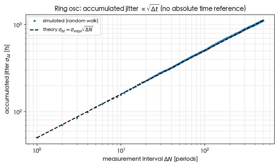
Toy parameters: $f_0=5$ GHz, $\sigma_{edge}=50$ fs/transition, 2000 trials. Full script: simulations/lab_03_ring_toy_model.py (fig_accumulation).

Step 4: what the ISF can and cannot see

Visible (ISF framework's strength)	Invisible / needs other treatment
Distribution of phase sensitivity vs. injection phase ($\Gamma$ shape)	Absolute value of tank $Q$, inductor parasitics (needs circuit model)
white→1/f², flicker→1/f³ scaling	Strong nonlinearity, large-signal AM-PM effects (first-order ISF insufficient)
Symmetry→$c_0$→1/f³ corner	Supply/substrate coupling ([P2] treats this qualitatively in a separate section)
Relative leverage of $\Gamma_{rms}$, $q_{max}$	Real $\Gamma$ shape (needs transient/adjoint extraction)
Accumulated jitter random walk	Exact $\kappa$, absolute value of FOM constant (needs a full device model; the formula itself is [P2] Eq.(12)/(23), verified)

Design knobs (LC vs ring comparison)

Goal	LC knob	Ring knob
Lower phase noise (1/f²)	Increase tank $Q$, increase swing ($q_{max}$)	Increase per-stage current/swing; single-ended: $N$ almost no effect; differential: fewer $N$ is better (Eq.34, see Step 2b)
Lower 1/f³ (close-in)	Symmetric differential, low $c_0$	Symmetric load ([P2] Fig. 17 symmetry voltage)
Wide tuning	Varactor (narrow range)	Change bias current/$\tau_D$ (wide range, ring's strength)
Multiphase output	Needs extra circuitry	Inherently $N$ phases (ring's strength)
Small area	Large (spiral inductor)	Small (ring's strength)

Worked numerical examples

The following two examples use [P2]'s ring white-noise FOM to compute a concrete $\mathcal{L}$, and verify that "at fixed $f_0$/power, phase noise is roughly independent of $N$." The formulas have been verified against the original [P2] PDF; below we take $\eta\approx1$ (stage-delay proportionality constant, entering the prefactor $8/(3\eta)$), $\gamma=2/3$ (long channel, entering only through $V_{char}=\Delta V/\gamma$), $V_{DD}/V_{char}=3$ (illustrative value); the numbers are an order-of-magnitude demonstration.

Example 1 (use the ring FOM to compute 1/f² phase noise, comparing N=3/5/15) Take $f_0=5$ GHz, offset $\Delta f=1$ MHz, $kT=4.0\times10^{-21}$ J (300 K), $P=1$ mW, $\eta\approx1$, $\gamma=2/3$ (already absorbed into $V_{DD}/V_{char}=3$). Compute $\mathcal{L}|_{1/f^2}$ using [P2] Eq.(23); $N$ does not appear explicitly in this expression (already absorbed by N-independence), so N=3/5/15 give the same value.

Step-by-step substitution (with units), using $\mathcal{L}|_{1/f^2}=\dfrac{8}{3\eta}\dfrac{kT}{P}\dfrac{V_{DD}}{V_{char}}\Big(\dfrac{f_0}{\Delta f}\Big)^2$:

$$\begin{aligned} \frac{f_0}{\Delta f}&=\frac{5\times10^9}{1\times10^6}=5000,\quad \left(\frac{f_0}{\Delta f}\right)^2=2.5\times10^{7}, \\[4pt] \frac{kT}{P}&=\frac{4.0\times10^{-21}\ \text{J}}{1\times10^{-3}\ \text{W}}=4.0\times10^{-18}\ \text{s}, \\[4pt] \frac{8}{3\eta}&=\frac{8}{3}\approx2.667\quad(\eta\approx1),\qquad \frac{V_{DD}}{V_{char}}=3, \\[4pt] \text{bracket}&=2.667\times3\times(4.0\times10^{-18})\times(2.5\times10^{7})=8.0\times(4.0\times10^{-18})\times(2.5\times10^{7})=8.0\times10^{-10}, \\[4pt] \mathcal{L}|_{1/f^2}&=10\log_{10}(8.0\times10^{-10})=-91.0\ \text{dBc/Hz}. \end{aligned}$$

• Result: $\mathcal{L}|_{1/f^2}\approx-91.0$ dBc/Hz @ 1 MHz — identical for N=3, N=5, N=15, because at fixed $f_0$/$P$ the $N$-dependent factors cancel (claim C7). This is $\sim57$ dB worse than example 2's ideal LC value ($-148$ dBc/Hz), which is reasonable order-of-magnitude: ring has no high-$Q$ energy storage, small $q_{max}$, and many devices.
• Dimension check: $\dfrac{[\text{J}]}{[\text{W}]}\cdot(\text{dimensionless})^2=\dfrac{[\text{J}]}{[\text{J/s}]}=[\text{s}]$, the per-Hz power ratio ($1/\Delta\omega^2$ already absorbed into $(\omega_0/\Delta\omega)^2$) → $10\log_{10}$ gives dBc/Hz ✓.
• One-line Python check:

import numpy as np
def L_ring_fom(kT, P, f0, df, eta=1.0, vdd_vchar=3.0):   # [P2] Eq.(23), prefactor 8/(3*eta)
    return 10*np.log10(8/(3*eta) * (kT/P) * vdd_vchar * (f0/df)**2)
vals = {N: L_ring_fom(4.0e-21, 1e-3, 5e9, 1e6) for N in (3, 5, 15)}
print({N: round(v,1) for N,v in vals.items()})    # -> {3: -91.0, 5: -91.0, 15: -91.0}

N-independence here is a direct consequence of "Eq.(23) simply contains no $N$" — and the toy exponents agree: $\Gamma_{rms}^2\propto N^{-3}$ (Eq.16), $q_{max}\propto N^{-1}$ (from Eq.(21) at fixed $P$, $f_0$), and $\times N$ noise sources, so $\Gamma_{rms}^2/q_{max}^2\cdot N\propto N^{-3+2+1}=N^0$, consistent with Eq.(23) (see lab_17 for the walkthrough).

Example 2 (LC vs ring: how much better is LC under comparable-order conditions?) Use [P1] Eq.(21) to compute a representative LC number and place it side by side with ring's $-91.0$ dBc/Hz above. Take canonical $\Gamma_{rms}=0.5$, $q_{max}=1$ pC, $S_i=\overline{i_n^2}/\Delta f=10^{-24}$ A²/Hz, $f_0=5$ GHz, $\Delta f=1$ MHz.

Step-by-step substitution (with units), using [P1] Eq.(21) $\mathcal{L}=10\log_{10}\!\big(\frac{\Gamma_{rms}^2}{q_{max}^2}\cdot\frac{S_i}{4\Delta\omega^2}\big)$:

$$\begin{aligned} \Delta\omega&=2\pi\times10^6=6.283\times10^6\ \text{rad/s},\quad \Delta\omega^2=3.948\times10^{13},\\[4pt] \text{bracket}&=\frac{0.25}{10^{-24}}\cdot\frac{10^{-24}}{4\times3.948\times10^{13}}=\frac{0.25}{1.579\times10^{14}}=1.583\times10^{-15},\\[4pt] \mathcal{L}_{LC}&=10\log_{10}(1.583\times10^{-15})=-148.0\ \text{dBc/Hz}. \end{aligned}$$

• Comparison: under ideal single-source conditions, LC $-148$ vs ring $-91$ → LC is about 57 dB better. (The two numbers come from each paper's own natural parametrization: LC uses $q_{max},\Gamma_{rms},S_i$, ring uses $P,\gamma,V_{DD}/V_{char}$, so this is an "order-of-magnitude comparison," not a same-parameter-set comparison. Real-world gaps are often 10-30 dB, because ring has multiple noise sources, cyclostationary effects, and flicker.) This quantifies "LC buys low phase noise with high-$Q$ energy storage."
• Dimension check: same as [P1] Eq.(21) (see white_noise_to_phase_noise), bracket is dimensionless ✓.
• One-line Python check:

import numpy as np
def L_lc(Grms, qmax, Si, f0, df):                 # [P1] Eq.(21)
    dw = 2*np.pi*df
    return 10*np.log10(Grms**2/qmax**2 * Si/(4*dw**2))
print(round(L_lc(0.5, 1e-12, 1e-24, 5e9, 1e6), 1))   # -> -148.0

The above [P2] constants (prefactor $8/(3\eta)$, $\Gamma_{rms}=\sqrt{2\pi^2/(3\eta^3)}\cdot N^{-1.5}$, Eq.(23) FOM) have all been verified against the original PDF; the only conclusion that is solid and directly usable for design is N-independence itself and the $N^0$ exponent cancellation. Full script: simulations/lab_03_ring_toy_model.py.

Key takeaways

• LC: sinusoidal waveform, $\Gamma=-\sin$, high-$Q$ energy storage, large $q_{max}$, few devices, low phase noise, slow jitter accumulation.
• ring: square wave, ISF concentrated at transition, no energy storage, $N$ noise sources, $\Gamma_{rms}\propto N^{-3/2}$, fast random-walk jitter.
• [P2]'s three formulas: $f_0=1/(2N\tau_D)$ (Eq.15), $\Gamma_{rms}\propto N^{-3/2}$ (Eq.16, re-verified in v7: the radical covers only the constant), FOM $\frac{8}{3\eta}\,\frac{V_{DD}}{V_{char}}\,\frac{kT}{P}(\omega_0/\Delta\omega)^2$ (Eq.23, prefactor $8/(3\eta)$, verified).
• N-independence: at fixed $f_0$/power, ring phase noise is roughly independent of $N$ ($N$-dependent factors cancel); choose $N$ based on tuning/multiphase/area.
• Differential-ring exception: [P2] Eq.(34), p.796 contains an explicit $N$ — at fixed $f_0$/power, $\mathcal{L}$ degrades as $10\log_{10}N$ (the culprit is $q_{max}\propto1/N^2$); $N=4\to12$ costs $+4.77$ dB. Differential designs should use the fewest necessary stages.
• The ISF sees the distribution and scaling of phase sensitivity; it cannot see absolute $Q$, strong nonlinearity, coupling, or exact constants.

Further reading

• ring lab: lab_03_ring_oscillator_toy_model
• LC lab: lab_02_lc_oscillator_toy_model
• What LC's "high-$Q$ energy storage" actually buys ($Q$'s three definitions, $-R$ compensation, $4kT/R_p$): tank_Q_and_energy_restoration
• Phase noise from tuning/supply jitter (LC-VCO's other major noise entry point): varactor_tuning_supply_pushing
• $\Gamma_{rms}$: rms_isf; swing: tank_swing
• Symmetry: symmetry; slope: waveform_slope
• Jitter and SerDes: serdes_clocking_connection